
Price elasticity models, markdown timing, and inventory aging signals — the hidden analytics stack behind every promotional decision on the shelf.
You walk into a grocery store on a Tuesday afternoon and notice that your favorite brand of pasta sauce has a bright yellow "25% OFF" sticker slapped on it. You grab three jars instead of one. Deal won. But here's what you didn't see: a data scientist, somewhere in a corporate office, ran a model three weeks ago that told a merchandising manager exactly when to apply that discount, at what percentage, and for how long — before a single jar started collecting dust. The markdown wasn't reactive. It was a calculated prediction, and you walked right into it. This is the hidden analytics stack behind every promotional shelf decision in modern retail. And it's far more sophisticated than most people — including many early-career data scientists realize.
The Foundation: Price Elasticity Isn't One Number
Most textbooks introduce price elasticity of demand as a single coefficient: the percentage change in quantity demanded divided by the percentage change in price. Clean, simple, and almost entirely useless in production retail. Real-world price elasticity is a function, not a constant. It varies across:
- Customer segments — price-sensitive shoppers respond differently than brand-loyal buyers
- Time of week and season — a 10% discount on charcoal hits different in July than in November
- Competitive context — your elasticity collapses when a competitor runs a deeper promotion simultaneously
- Category role — commodities (cooking oil, eggs) have very different elasticity curves than aspirational products (premium coffee, craft beer)
The practical modeling approach most retail analytics teams use is a log-log regression with interaction terms, sometimes extended into a mixed-effects framework when product hierarchies matter:
log(Qty) = β₀ + β₁·log(Price) + β₂·log(CompetitorPrice) + β₃·Promo + β₄·Season + ε
Here, β₁ is your base elasticity estimate, but the real insight lives in β₃ and β₄ — the interactions that tell you when a price move will actually move volume versus just eroding margin. Teams that skip these interactions end up over-discounting in periods where demand would have been strong anyway, essentially leaving money on the table by giving away margin they didn't need to. The output isn't just "this product is elastic at -1.8." It's a curve that says: dropping price by 10% during back-to-school week in the pasta sauce category drives a 24% volume lift, but the same move in the first week of December only drives 9%. That's the intelligence that feeds the markdown engine.
Markdown Timing: The Inventory-Demand Intersection
Knowing elasticity is necessary but not sufficient. The harder question is when to pull the trigger on a discount — and that's where inventory aging signals come in. Every product sitting in a warehouse or on a shelf has an implicit clock running against it. For perishables, it's obvious. For general merchandise, it's subtler but equally real: carrying costs, storage fees, capital tied up in unsold inventory, and the risk of obsolescence (especially in fashion and electronics) all compound over time. The markdown timing problem is essentially an optimization question:
What is the optimal price reduction, applied at what point in the product lifecycle, that maximizes total revenue (or margin) while clearing inventory before it becomes a liability?
The core signal retailers watch is weeks of supply (WOS) relative to expected sell-through velocity:
WOS = Current Inventory / Average Weekly Sales Rate
When WOS exceeds a category-specific threshold — say, 8 weeks for seasonal apparel with a 12-week selling window — that triggers an automated markdown recommendation. But the recommendation isn't just "discount it." It's a staged markdown schedule: perhaps 15% off in week one to test demand response, followed by 25% if velocity doesn't recover, then a deeper clearance cut as the deadline approaches. What makes this genuinely hard is that the markdown itself changes the sell-through velocity, which changes the WOS projection, which changes whether you needed to go deeper. You're solving a dynamic problem with a feedback loop, not a static one. Teams that treat it as static consistently either over-discount (clearing too fast, destroying margin) or under-discount (missing the window and ending up with clearance inventory anyway, just at worse timing).
The Inventory Aging Signal Stack
Beyond WOS, sophisticated retailers build what's internally called an aging signal stack — a composite of features that together predict whether a product is heading toward a markdown situation before the inventory numbers make it obvious.
The key signals typically include:
Velocity decay rate — how much has weekly sales velocity declined over the past 4 weeks relative to the product's historical baseline? A product sitting at -30% velocity decay is a markdown candidate, even if absolute inventory looks fine.
Demand-supply ratio trend — not just current ratio, but whether it's been improving or deteriorating week over week. A product with a deteriorating ratio at 1.2x is more concerning than one sitting stable at 0.9x.
Substitution pressure — are similar products in the category seeing a velocity uptick? This often signals that a competitor or private label is stealing share, making your inventory position worse than the raw numbers suggest.
Promotional calendar proximity — a product with aging inventory three weeks before a major category event (back-to-school, holidays) might benefit more from holding price and riding the seasonal lift than taking a markdown that compresses future margin.
When you stack these signals together as features into a gradient boosted model, you get a markdown probability score for each SKU every week. Scores above a threshold route automatically to a merchandising analyst for review and action. Scores approaching a critical threshold trigger alerts. This is how a retailer with 30,000 SKUs can manage promotional decisions that would be humanly impossible to handle manually.
Where the Models Break (And What Practitioners Do About It)
No production retail analytics system runs perfectly, and understanding where these models fail is what separates a strong data scientist from a great one.
New product introductions are the most common failure mode. Elasticity models need historical price-volume data. A brand-new SKU has none. Most teams solve this with a cold-start approach: borrowing elasticity priors from the most similar existing product in the category, then updating as the first 8–12 weeks of data accumulate. It's imperfect, but far better than applying a category average blindly.
External shocks break velocity baselines. A viral social media moment, a news event tying to a category, a supply chain disruption at a competitor — these all cause sudden, non-seasonal volume spikes or drops that make historical averages poor predictors. The practical fix is anomaly detection on the input features: when velocity deviates more than 2–3 standard deviations from its rolling baseline, flag the model's recommendation for human review rather than acting on it automatically.
Cannibalization is the sleeper issue. When you run a promotional discount on one SKU in a category, you often pull volume from adjacent SKUs at full price. A model optimizing the promoted SKU's margin in isolation looks great; a model that accounts for category-level margin often recommends a shallower discount because the cannibalization effect eats into gains on the rest of the shelf. This is why the best retail analytics teams model at the category level, not the SKU level alone.
What This Looks Like in a Real System
In practice, a mature retail analytics stack for promotional decision support looks something like this: weekly transaction data flows into a feature engineering pipeline that computes elasticity inputs, aging signals, and competitive context. These feed a set of models — price response, markdown probability, cannibalization estimates — whose outputs are combined into a recommendation engine. Recommendations surface in a merchandising dashboard with confidence intervals and override controls, because experienced merchants know things the model doesn't (like a vendor relationship that makes a specific markdown inadvisable, or a local market nuance that skews the national model).
The data scientist's job isn't to automate away the merchant. It's to give the merchant a decision support system that lets them make 300 high-quality promotional calls a week instead of 30 mediocre ones.
The Takeaway for Data Professionals
If you're building skills for retail analytics, the temptation is to focus on the models themselves — gradient boosted trees, mixed-effects regression, time series forecasting. Those matter. But the practitioners who create real business impact understand something deeper: the value isn't in the model's accuracy. It's in the system's ability to convert a signal (aging inventory) into a decision (markdown timing) into a business outcome (margin-preserving sell-through) at scale. The next time you see a yellow discount sticker on a shelf, know that it's not a gut-feel call. It's the output of a probability score that ran last Wednesday, ranked against 30,000 other SKUs competing for the same promotional budget — and the data said your pasta sauce was ready.
--- This post is part of DSBootcamp's Retail Analytics series, where we break down the real analytics systems powering enterprise decisions — with the business context, modeling approaches, and failure modes that production work actually demands. ---