From statistical baselines to ML overrides — how large retail teams combine human judgment and algorithmic forecasting to decide how much of every SKU to order every week.
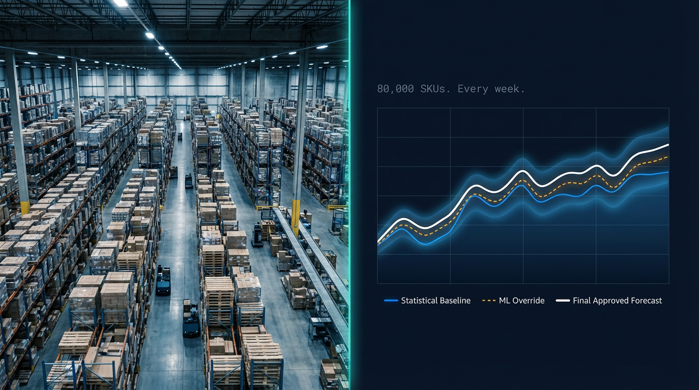
Here is a number worth sitting with for a moment: a large-format retailer carrying 80,000 active SKUs across 400 stores needs to make roughly 32 million individual replenishment decisions every week. Not every month. Every week. How many units of each product to order, for each location, accounting for lead times, promotional calendars, seasonal curves, supplier constraints, and the simple reality that consumer behavior is not a fixed equation.
No human team can do this manually. But no algorithm, no matter how sophisticated, can do it alone either. What actually runs demand forecasting at a Fortune 500 retailer is a carefully engineered hybrid — statistical baselines that handle the predictable bulk of the problem, machine learning layers that capture complexity those baselines miss, and human override workflows that inject judgment where models are structurally blind.
Understanding how these three layers interact is one of the most practically valuable things a retail data scientist can learn. This is how it actually works.
Why the Problem Is Harder Than It Looks
The naive framing of demand forecasting is: look at last year's sales, adjust for growth, and order accordingly. Some retailers still operate close to this model. They tend to have chronically overstocked warehouses in slow periods and persistent stockouts during peak demand, with margin erosion on both ends.
The real problem is harder for several compounding reasons.
Demand is not stationary. Consumer preferences shift, competitor promotions disrupt baselines, economic conditions alter category-level spending, and new product introductions cannibalize existing ones. A forecast built on a fixed historical window without accounting for these structural breaks will drift systematically in the wrong direction.
Promotions distort the signal. A SKU that ran a 20% promotion for three weeks last year has inflated historical demand in exactly those weeks. If your forecast naively includes those promoted weeks in its baseline, it will over-order in the same period this year and create excess inventory that requires markdowns to clear. Promotional lift must be modeled separately and stripped from the baseline before the baseline can be trusted.
Lead times create forecast horizons that amplify error. If your supplier requires a 6-week order lead time, you're not forecasting next week — you're forecasting six weeks from now, for delivery in the seventh week. Forecast error compounds with horizon length. A 10% error at a one-week horizon might translate to a 25–30% error at a six-week horizon, and the inventory consequences of that error are proportionally larger because you've committed to a larger order.
The long tail is enormous. The top 500 SKUs in a large retailer's assortment might represent 40% of revenue and are relatively easy to forecast — they have long history, stable velocity, and enough sales volume to make statistical patterns robust. The remaining 79,500 SKUs are where most of the operational pain lives: slow movers, regional specialties, new introductions, and seasonal items with short selling windows and thin historical data. The methods that work well on the top of the assortment often fail entirely on the tail.
This is the landscape that a production forecasting system has to navigate, at scale, every week.
Layer One: The Statistical Baseline
Every mature demand forecasting system starts with a statistical baseline model. Its job is not to be the best possible forecast — it's to be a reliable, explainable, computationally efficient floor that handles the majority of SKUs adequately and provides a foundation that more complex layers can build on.
The workhorse of statistical baseline forecasting in retail is Holt-Winters exponential smoothing (also called Triple Exponential Smoothing), extended with promotional and calendar adjustment factors. It handles trend and seasonality natively, updates continuously as new sales data arrives, and is fast enough to run across hundreds of thousands of SKUs without prohibitive compute cost.
The core update equations balance recent observations against historical patterns using smoothing parameters:
Level: Lₜ = α(Yₜ / Sₜ₋ₘ) + (1 - α)(Lₜ₋₁ + Tₜ₋₁)
Trend: Tₜ = β(Lₜ - Lₜ₋₁) + (1 - β)Tₜ₋₁
Season: Sₜ = γ(Yₜ / Lₜ) + (1 - γ)Sₜ₋ₘ
Where Yₜ is observed demand, m is the seasonality period, and α, β, γ are the smoothing parameters tuned per SKU or category. The forecast at horizon h is then:
Ŷₜ₊ₕ = (Lₜ + h·Tₜ) × Sₜ₋ₘ₊ₕ
Before this model ever sees raw sales data, the data must be cleaned. Promotional periods are flagged and either removed from the baseline fitting window or adjusted using a pre-estimated promotional lift factor. Stockout periods — weeks where zero sales were recorded because inventory was unavailable, not because demand was zero — must be imputed rather than fed as genuine demand signal. Feeding zero demand from a stockout week into a forecasting model is one of the most common data quality errors in retail forecasting systems, and it systematically biases baseline forecasts downward in categories with frequent availability issues.
The output of the statistical baseline is a clean, adjusted demand forecast for each SKU at each location for the required planning horizon. For the majority of stable, mature SKUs with adequate sales history, this baseline is already good enough to drive replenishment decisions. The problems start at the edges — and that's where the ML layer begins.
Layer Two: The Machine Learning Override
The statistical baseline is excellent at capturing what a product's demand pattern has looked like historically. It's structurally limited at capturing what will make demand behave differently in the future. That's the specific problem machine learning is deployed to solve in a production forecasting stack.
The ML layer in most sophisticated retail forecasting systems isn't a single model replacing the baseline. It's a set of targeted override models that operate on specific forecast failure modes. Here are the three most common:
Promotional lift modeling. When a promotion is planned for a future week, the baseline doesn't know how to adjust the forecast — it only knows what happened in prior promotional events, and those events are stripped from the baseline training data. A gradient boosted model trained on historical promotional events, with features including discount depth, promotional mechanic (buy-one-get-one vs. percentage off vs. featured placement), competitive promotion context, seasonality timing, and category, can produce a promotional lift multiplier that adjusts the baseline forecast for the planned promotional period. This is one of the highest-ROI applications of ML in retail forecasting because promotional weeks concentrate a disproportionate share of both volume and margin exposure.
New product forecasting. A brand-new SKU has no sales history. The statistical baseline cannot run. The ML approach is a similarity-based cold start: embedding the new product in a feature space defined by category, price tier, brand, package size, and supplier, then finding the most similar historical products and using their early-lifecycle velocity curves as the prior forecast. The model is updated rapidly as the first 4–8 weeks of actual sales data arrive, transitioning from the similarity-based prior to a data-anchored estimate.
Anomaly and external signal integration. Baseline models and standard promotional models don't capture signals that exist outside the retailer's own transaction history — weather forecasts, social media trend velocity, economic indicators, competitor pricing data, or local events. An ML layer can ingest these external signals as features and produce forecast adjustments for specific SKU-location combinations where the signal is relevant. Ice cream demand before a forecasted heat wave. Generator sales before a major storm. Flu medication demand correlated with CDC flu tracker data in specific geographies. These are cases where external signal integration can meaningfully outperform a history-only model.
The ML override layer produces adjustment factors — multipliers or additive corrections — applied to the statistical baseline rather than replacing it. This design choice is deliberate. It means the baseline remains interpretable, the ML contribution is auditable, and a failure in the ML model degrades gracefully rather than catastrophically corrupting the entire forecast.
Layer Three: Human Override Workflows
Here is the part that surprises most people who come to retail forecasting from a pure data science background: in a well-run retail forecasting operation, human override capability isn't a workaround for model inadequacy. It's a designed feature of the system.
Algorithms are trained on historical data. They are, by construction, blind to information that doesn't yet exist in structured form in a database. Category managers and merchants carry a constant stream of forward-looking, unstructured intelligence that no model sees: a supplier just called to warn about a 3-week shipment delay. A competitor announced a store closure in three of your trade areas. A major influencer posted about a product in your assortment yesterday and the DMs are already coming in. An unusual weather pattern is tracking toward your highest-index coastal stores during a key seasonal period.
This is the information that makes experienced human judgment genuinely additive to algorithmic forecasting — not as a substitute for the model, but as a layer on top of it.
Production forecasting systems handle this through a structured exception workflow. The forecasting engine runs automatically and routes the outputs to planners. Planners see the system forecast alongside a confidence interval and a set of exception flags: items with high forecast volatility, new products approaching their baseline transition threshold, items with planned promotions whose lift model has high uncertainty, items flagged by the ML anomaly layer as having unusual external signals. The planner reviews exceptions, applies overrides where their judgment diverges from the model, documents the reason, and approves the forecast for the replenishment engine.
The override documentation is critical — not just for accountability, but because it creates a labeled training dataset. Override events, tagged with their documented reason, can be used to identify systematic model gaps. If a planner is consistently overriding the forecast for a specific category upward before weather events, that's a signal that a weather feature belongs in the ML layer for that category. Human overrides, treated analytically, become a roadmap for model improvement.
The best forecasting teams track override accuracy as a first-class KPI: when a planner overrides the system forecast, is the planner's override more accurate than what the model would have produced? Teams that measure this consistently discover that human overrides are not uniformly valuable. Some planners reliably add accuracy in specific domains. Others introduce systematic bias — over-optimism on new products, under-adjustment for promotional cannibalization. This analysis is sensitive but important, because it directly affects how much authority the human override layer should carry in the system design.
The Forecast Accuracy Measurement Problem
A forecasting system is only as good as your ability to measure its performance accurately, and retail forecast accuracy measurement has several non-obvious traps.
MAPE (Mean Absolute Percentage Error) is the most commonly reported forecast accuracy metric in retail, and it's deeply problematic for slow-moving SKUs. When actual demand is very low — say, two units per week for a regional specialty product — a forecast of three units produces a 50% error. The absolute impact is one unit, but the percentage makes it look like a catastrophic failure. Teams that optimize for MAPE end up over-investing model complexity in low-volume SKUs where the business impact is small, while under-attending to high-volume SKUs where a smaller percentage error represents massive absolute exposure.
Weighted MAPE (weighting the error by revenue contribution) is a significant improvement, but it still doesn't capture the asymmetric cost of forecast error. An overforecast by 10% leads to excess inventory and carrying cost. An underforecast by 10% leads to stockouts and lost revenue. These costs are not equal, and the relative magnitudes vary by category, seasonality, and product lifecycle stage. Sophisticated forecasting teams build asymmetric loss functions that penalize underforecasting more heavily in high-velocity, high-margin categories and overforecasting more heavily in perishable or fashion categories approaching the end of their selling window.
Naive benchmarking is the practice of always measuring forecast accuracy against a naive baseline — typically last year's actuals or a simple moving average. A forecast system that uses a sophisticated ML stack but only marginally outperforms a last-year baseline on most SKUs is an expensive infrastructure investment with limited incremental value. Every reporting dashboard in a mature forecasting operation should show the ML forecast accuracy alongside the naive benchmark, forcing the team to continuously justify the complexity.
What the Full Stack Actually Looks Like
In a mature Fortune 500 retailer, the demand forecasting infrastructure looks roughly like this end-to-end.
Weekly sales, inventory, and promotional data flows into a centralized data platform — typically a cloud data warehouse running on Snowflake, Databricks, or a comparable platform. A data quality pipeline flags stockout periods, anomalous transaction spikes, and data latency issues before any model sees the data. The statistical baseline model runs at the SKU-location level, producing a clean adjusted baseline forecast. The ML override models run in parallel, ingesting external signals and producing adjustment factors. The combined forecast, with confidence intervals, surfaces in a planner-facing dashboard with exception prioritization. Planner overrides and approvals feed back into the system. The approved forecast triggers the replenishment engine, which converts demand forecasts into purchase orders via order quantity optimization that accounts for supplier minimum order quantities, pallet configurations, lead time variability, and service-level targets.
The cycle repeats weekly. The models retrain on a rolling basis. Override accuracy is tracked. External signal sources are evaluated and rotated. The system is never finished — it's a continuously improving operational infrastructure.
What This Means If You're Building Retail Analytics Skills
Demand forecasting is one of the most important and most complex problems in retail analytics, and it's one where understanding the business system is as important as understanding the modeling techniques. The data scientists who create the most value in this domain aren't necessarily those with the most sophisticated ML toolkit — they're the ones who understand why the statistical baseline exists alongside the ML layer, who design their ML overrides to degrade gracefully, who treat human override data as a model improvement signal, and who measure forecast accuracy in a way that actually reflects business impact.
The 32 million decisions that need to happen every week don't get better by making the models more complex. They get better by making the entire system — data, models, human judgment, and measurement — more coherent.
That's what running forecasting at scale actually means.
---
This post is part of DSBootcamp's Retail Analytics series, where we break down the real systems and decision frameworks powering enterprise retail operations — built for data scientists who want to understand the domain as deeply as the data.
---