Skewed outcomes, multiplicative effects, interpreting log-linear regression coefficients, and the geometric mean as the right summary statistic for log-transformed data.
Revenue. Salary. Transaction value. Time on site. Inventory cost. Customer lifetime value.
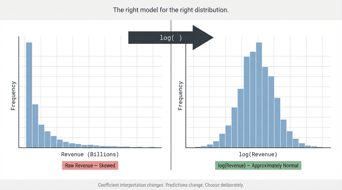
Every one of these is a canonical outcome variable in business analytics. Every one of them shares the same distributional character: strictly positive, right-skewed, spanning multiple orders of magnitude. A company's revenue distribution doesn't have a cluster of observations at $0 and a symmetric bell curve above it. It has a large mass of small-to-mid values and a long tail of outliers that can be ten, fifty, or a hundred times larger than the median.
The standard move — and the correct one in most of these cases — is to model the log of the outcome rather than the outcome itself. But this recommendation is often applied as a reflex rather than a reasoned decision, and when practitioners don't understand why the log transformation works, they also don't know when it doesn't, and they routinely misinterpret the coefficients of the models they build.
This post covers the reasoning, the mechanics, and the interpretive discipline that log-transformed regression requires.
Why Skewed Outcomes Break OLS Assumptions
Ordinary least squares regression finds the line that minimizes the sum of squared errors. When the outcome variable is heavily right-skewed, a small number of extreme observations generate enormous squared errors that the model works disproportionately hard to reduce — at the expense of fitting the bulk of the distribution well. The result is a model whose predictions are pulled toward the outliers, whose residuals are systematically non-normal (violating the assumption that validates standard errors and hypothesis tests), and whose predictions on held-out data are unstable.
The more fundamental issue is structural. Linear regression models additive effects: a one-unit increase in X produces a β unit increase in Y, regardless of the current level of Y. For many business processes, this is the wrong functional form. A 10% discount doesn't produce a fixed-dollar lift in sales — it produces a percentage lift proportional to the current sales level. A senior hire doesn't earn exactly $50,000 more than a junior hire — they earn a percentage premium. Marketing spend doesn't add a fixed number of customers — it multiplies the existing customer acquisition rate by some factor.
These are multiplicative processes, and the natural model for a multiplicative process is a log-linear regression.
The Log-Linear Model and What It Actually Says
When you regress log(Y) on X:
log(Y) = β₀ + β₁X + ε
The interpretation of β₁ changes fundamentally. It is no longer "a one-unit increase in X produces β₁ more units of Y." It is "a one-unit increase in X is associated with an approximate β₁
× 100 percent change in Y."
More precisely, for continuous X:
% change in Y ≈ (e^β₁ − 1) × 100
The Geometric Mean: The Right Summary Statistic After Log-Transformation
Here is where most practitioners make a subtle but consequential error. After fitting a log-linear model and obtaining predictions on the log scale, they exponentiate those predictions to get back to the original scale. What they get is the geometric mean prediction of Y — not the arithmetic mean prediction. They are not the same thing, and conflating them understates the predicted value for skewed distributions.
The relationship between the two is governed by the variance of the log-transformed residuals:
E[Y] = exp(μ_log + σ²/2) ← Arithmetic mean (what you probably want for revenue totals) Median[Y] = exp(μ_log) ← Geometric mean (what exp(ŷ) gives you)
Where μ_log is the mean on the log scale and σ² is the variance of the log-scale residuals. For a lognormal distribution, the arithmetic mean is always larger than the geometric mean — sometimes substantially so when variance is high.
Use the geometric mean prediction when: you want predictions that represent the typical individual observation — the median, essentially. Customer LTV for individual targeting decisions. Expected revenue for a single SKU in a single store. The central tendency of one transaction.
Use the arithmetic mean prediction (with smearing) when: you're aggregating. Forecasting total revenue across 10,000 customers. Estimating total category sales. Any context where you're summing predictions across a population. Geometric mean predictions will systematically underestimate aggregated totals for right-skewed outcomes, sometimes by large margins when variance is high.
The practical rule: individual predictions use geometric mean; aggregate predictions use arithmetic mean with the smearing correction. Applying the wrong one to the wrong context is a quiet, consistent source of forecast error in production systems.
When You Should Not Log-Transform
The log transformation is powerful and appropriate in many contexts. It is not universally correct, and applying it reflexively creates its own problems.
When the outcome contains zeros or negatives. The natural log is undefined at zero and imaginary for negative values. log(Y + 1) is a common workaround, but it changes the interpretation of the model and can produce misleading results when there are many zeros relative to the range of positive values. For outcomes with structural zeros — customers who made no purchase, stores with no sales in a given week — consider a two-part model: one model for the probability of a non-zero outcome, and a separate log-linear model for the magnitude conditional on being non-zero.
When the effect you're modeling is genuinely additive, not multiplicative. Not every business process is multiplicative. Temperature increase and energy consumption. Headcount and payroll cost. Unit price and item margin. When the theoretical relationship between X and Y is genuinely linear — each additional unit of X produces the same absolute increment in Y regardless of the current Y level — a log transformation misspecifies the model. The residual plot from an untransformed linear model is the diagnostic: if residuals are randomly scattered around zero with no fan shape, the linear model fits well and the log transformation is unnecessary.
When you need predictions that are easy to communicate in the original scale. Log-linear models are correct. They are also harder to explain to non-technical stakeholders than linear models. A coefficient of 0.12 that means "12.7% increase" requires an exponentiation step that breaks in stakeholder presentations if not carefully handled. If your primary audience is a business team that will directly interpret the model output, the interpretive cost of log-transformation needs to be weighed against the statistical benefit.
When the outcome spans a narrow range with low skewness. If your outcome variable has a coefficient of variation below 0.3 and minimal tail behavior, the gain from log-transformation is marginal. Run both models, compare residual diagnostics, and choose based on fit quality rather than default habit.
The Decision Framework
Before deciding whether to log-transform your outcome, run through four checks:
1. Plot the distribution of Y
2. Check for zeros and negatives
3. Assess the theoretical data-generating process
4. Fit both models and compare residual diagnostics
The Interpretive Discipline the Log Transform Demands
A log-linear model demands one discipline above all: you must not interpret coefficients as if the model were linear. A coefficient of 0.15 does not mean "0.15 more dollars of revenue per unit increase in marketing spend." It means "15.3% more revenue per unit increase in marketing spend." These are completely different claims, and the second one scales with the current revenue level in a way the first does not.
Exponentiate every coefficient before presenting it. Always. Build the habit of reporting (exp(β) − 1) × 100 as the percentage change interpretation alongside the raw coefficient, and never let a log-scale coefficient appear in a stakeholder document without that translation. The model is only as useful as the interpretation it enables — and a misread log-linear coefficient is one of the most common and most quietly persistent errors in applied business regression.
This post is part of DSBootcamp's Statistics series, where we cover the modeling choices, statistical assumptions, and interpretive frameworks that make business regression analysis credible and actionable.