Residual plots, heteroscedasticity checks, multicollinearity via VIF, influential point detection, and what to do when assumptions break.
A regression model that fits your training data well is not the same thing as a regression model you can trust. This distinction sounds obvious when stated directly. It is violated constantly in practice.
The R² score on your holdout set tells you how much variance the model explains. It tells you nothing about whether the model's assumptions are met, whether its coefficients are stable, whether a handful of extreme data points are steering the entire fit, or whether the standard errors underlying your confidence intervals are valid. All of these can be badly wrong while your R² looks perfectly acceptable.
Trustworthiness in regression is not a single metric. It's a diagnostic process — a structured series of checks that together confirm the model is doing what you think it's doing, for the right reasons, in a way that will hold up under scrutiny. This is that process.
Why Regression Assumptions Actually Matter
Linear regression rests on a set of assumptions that are easy to state and surprisingly easy to violate without noticing:
- Residuals are approximately normally distributed
- Residuals have constant variance across predicted values (homoscedasticity)
- Features are not linearly dependent on each other (no multicollinearity)
- No single observation is exerting disproportionate leverage on the coefficients
- The relationship between features and target is actually linear
Violating these assumptions doesn't always destroy predictive accuracy — a model with heteroscedastic residuals might still predict reasonably well. What it destroys is the validity of everything built on top of the coefficients: hypothesis tests, confidence intervals, and the interpretation of individual feature effects. If you're using a regression model to make a causal claim — "a 10% increase in marketing spend drives a 3.2% lift in revenue" — and your assumptions are violated, that claim is not supported by your model, regardless of what the coefficient says.
For pure prediction tasks with no interpretive requirement, some violations matter less. For any model where the coefficients themselves are the output — pricing analysis, demand elasticity, A/B test estimation — they matter enormously. Know which type of model you're building before deciding how much rigor to apply.
Check 1: Residual Plots — The First Diagnostic You Run
Residuals are the difference between what your model predicted and what actually happened. If your model is well-specified, those errors should look like white noise — no pattern, no trend, no structure. Pattern in residuals means the model is systematically wrong in a detectable way.
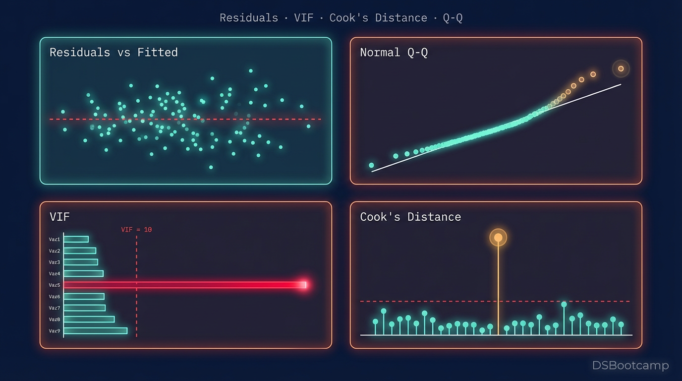
The core residual plot is fitted values on the x-axis, residuals on the y-axis. Run this before anything else.
import numpy as np
import matplotlib.pyplot as plt
from sklearn.linear_model import LinearRegression
from sklearn.model_selection import train_test_split
import statsmodels.api as sm

# Fit model using statsmodels for richer diagnostics
X_with_const = sm.add_constant(X_train)
model = sm.OLS(y_train, X_with_const).fit()

fitted_vals = model.fittedvalues
residuals = model.resid

# Residuals vs Fitted
plt.figure(figsize=(8, 5))
plt.scatter(fitted_vals, residuals, alpha=0.4, color='steelblue')
plt.axhline(0, color='red', linestyle='--')
plt.xlabel('Fitted Values')
plt.ylabel('Residuals')
plt.title('Residuals vs Fitted')
plt.tight_layout()
plt.show()
What healthy looks like: Points scattered randomly around zero, no systematic fan or curve shape, roughly equal spread across the range of fitted values.
What breaks look like:
A U-shaped or arched pattern means the relationship between a feature and the target is non-linear and your linear model is missing it. The fix is adding a polynomial term or transforming the feature.
A fan-shaped pattern — residuals spreading wider as fitted values increase — is heteroscedasticity. This gets its own dedicated check next because it's both common and consequential.
A wave pattern that repeats across fitted values suggests autocorrelation in the residuals, which is common in time-series data and violates the independence assumption. Check your data ordering if you see this.
Check 2: Heteroscedasticity — When Variance Isn't Constant
Heteroscedasticity means the variance of your residuals is not constant across the range of predictions. It's extremely common in business data — revenue models, for example, almost always have larger absolute errors at higher revenue values simply because the scale is larger.
The visual check is the residual plot described above. For a formal statistical test, the Breusch-Pagan test is the standard:
from statsmodels.stats.diagnostic import het_breuschpagan

bp_test = het_breuschpagan(model.resid, model.model.exog)
labels = ['LM Statistic', 'LM p-value', 'F-Statistic', 'F p-value']
results = dict(zip(labels, bp_test))
print(results)
A p-value below 0.05 on the Breusch-Pagan test rejects the null hypothesis of homoscedasticity — your residuals have non-constant variance, and your standard errors are unreliable.
What to do when heteroscedasticity is detected:
The first option is a log transformation of the target variable. If the target is revenue, price, counts, or anything strictly positive with a right-skewed distribution, log(y) often stabilizes variance dramatically. The interpretation shifts — your model now predicts log-revenue, and coefficients represent percentage changes rather than unit changes — but this is usually a better model of how the underlying process actually works.
The second option is robust standard errors (also called heteroscedasticity-consistent standard errors, or HC standard errors). These don't fix the heteroscedasticity — they adjust the standard error estimates to remain valid in its presence, preserving the validity of hypothesis tests without requiring a transformation.
The choice between these approaches depends on whether prediction or interpretation is the priority. Log transformation is usually better for prediction. Robust standard errors are often better when you need to preserve interpretability in the original scale.
Check 3: Normality of Residuals — The Q-Q Plot
The normality assumption matters most when your sample size is small or when you're relying on hypothesis tests for coefficient significance. With large samples, the Central Limit Theorem provides some protection, but checking is still worth the 30 seconds it takes.
The Q-Q (quantile-quantile) plot is the right tool. It compares the distribution of your residuals to a theoretical normal distribution. Points that fall on the 45-degree line are normally distributed. Deviations from the line reveal the specific character of the departure.
import scipy.stats as stats

fig, ax = plt.subplots(figsize=(6, 5))
stats.probplot(model.resid, dist="norm", plot=ax)
ax.set_title("Q-Q Plot of Residuals")
plt.tight_layout()
plt.show()
S-curves on the Q-Q plot indicate heavy tails — extreme values occur more often than a normal distribution would predict. Common in financial data and any outcome driven by rare large events.
Points pulling away only at one end indicate skewness. If the upper tail deviates upward from the line, your residuals are right-skewed — again, a target transformation often resolves this.
For a formal test alongside the visual, the Shapiro-Wilk test works well for sample sizes under a few thousand. For larger samples, virtually any non-trivial departure from normality will be statistically significant, making the visual check more informative than the p-value.
Check 4: Multicollinearity via VIF — Coefficient Stability
Multicollinearity inflates the variance of coefficient estimates, making them unstable and unreliable as measures of individual feature effects. A model with severe multicollinearity can have coefficients that flip sign or change magnitude dramatically with small changes to the training data — which means they should not be trusted as business insights regardless of how significant they appear.
VIF is the right diagnostic. Compute it on your final model's feature set:
from statsmodels.stats.outliers_influence import variance_inflation_factor

feature_names = X_train.columns.tolist()
vif_data = pd.DataFrame({
    'Feature': feature_names,
    'VIF': [variance_inflation_factor(X_train.values, i)
            for i in range(X_train.shape[1])]
}).sort_values('VIF', ascending=False)

print(vif_data)
VIF above 5 warrants investigation. VIF above 10 is a problem. The remediation approach is iterative: drop or combine the highest-VIF feature, recompute, repeat. The goal is not a model with zero multicollinearity — some correlation between features is normal and acceptable. The goal is a model where no feature's coefficient estimate is being substantially distorted by its relationships with others.
One important nuance: multicollinearity inflates variance but does not bias coefficient estimates. A high-VIF model is not giving you wrong answers — it's giving you unstable answers. The coefficient estimate might be directionally correct but numerically unreliable. If the goal is prediction only, this matters less. If the goal is using coefficients as business insights, this matters enormously.
Check 5: Influential Points — The Observations Steering Your Model
Influential points are observations that, if removed from the training set, would substantially change the model's coefficients. They are not the same as outliers — a point can be an outlier in the y-direction (unusual target value) without having much influence on the model, and a point can be highly influential without being an obvious outlier in any single variable.
There are two complementary measures:
Leverage measures how far an observation is from the center of the feature space. High-leverage points have unusual feature values. They have the potential to be influential, but not necessarily.
Cook's Distance measures actual influence: how much do the coefficients change if this point is removed? It combines leverage and residual size into a single influence measure.
influence = model.get_influence()
cooks_d, p_values = influence.cooks_distance

# Plot Cook's Distance
plt.figure(figsize=(10, 4))
plt.stem(np.arange(len(cooks_d)), cooks_d, markerfmt=',', basefmt='grey')
plt.axhline(4 / len(X_train), color='red', linestyle='--',
            label=f'Threshold (4/n)')
plt.xlabel('Observation Index')
plt.ylabel("Cook's Distance")
plt.title("Cook's Distance — Influential Points")
plt.legend()
plt.tight_layout()
plt.show()

# Flag high-influence observations
threshold = 4 / len(X_train)
influential_idx = np.where(cooks_d > threshold)[0]
print(f"Influential observations: {len(influential_idx)}")
print(df_train.iloc[influential_idx])
When you find high Cook's Distance observations, the right response is almost never to automatically delete them. First, investigate: is this a data quality issue (entry error, system glitch, wrong unit of measurement)? If yes, fix or remove. Is it a genuinely unusual but real business event (a massive one-time promotional spike, a store that briefly operated as a distribution center)? If yes, consider whether it belongs in the training data for a model that will predict under normal operating conditions. Is it just an extreme but valid observation that your model isn't designed to handle well? Then acknowledge it, note the limitation, and consider whether a separate model for extreme cases is warranted.
The worst outcome is an influential point that is a data error that went undetected, whose removal would change a key coefficient by 30%. That has happened in published research and in production business models. Cook's Distance is one of the few tools that catches it systematically.
When Assumptions Break: A Decision Framework
Running these checks produces a set of diagnostic findings. Knowing what to do with them is where judgment enters.
Non-linearity in residuals: Add polynomial features, try a log or square root transformation on the relevant feature, or consider whether a non-linear model (gradient boosting, GAM) is more appropriate for the problem.
Heteroscedasticity: Log-transform the target if it's strictly positive and right-skewed. Apply robust standard errors if you need to preserve scale interpretability. Consider weighted least squares if you have domain knowledge about which observations should be down-weighted.
Non-normal residuals with large sample: Generally acceptable. The Central Limit Theorem covers coefficient estimates. Revisit if sample size is below a few hundred.
High VIF features: Drop one of the correlated pair, create a ratio or difference feature, or apply ridge regression which handles multicollinearity through regularization rather than removal.
Influential points from data errors: Fix or remove. Document the decision.
Influential points from real but extreme observations: Consider robust regression methods (Huber regression, quantile regression) that are less sensitive to extreme observations than OLS.
This post is part of DSBootcamp's Fundamentals series, where we cover the techniques every data scientist needs to know — with the rigor, code, and real-world context that production work actually demands.