Part 1 of 3 — The discipline, the problem it solves, and four foundational methods for recovering causation from data you didn't design.
Most data scientists are trained to build models that predict. Given this customer's behavior, what is the probability they churn? Given this product's features, what price will the market bear? Given this patient's history, what is the likelihood of readmission?
Prediction is valuable. But prediction answers a different question than the one that drives most business decisions. The business question is almost never "what will happen?" in isolation. It is almost always "what will happen if we do this?" — and that is a causal question, not a predictive one.
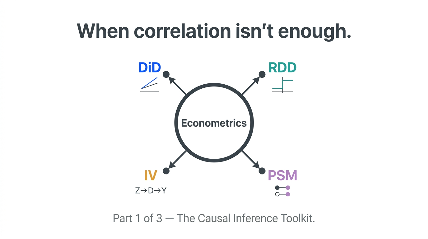
Econometrics is the discipline that takes causal questions seriously. It originated in economics as the science of estimating relationships in economic data — quantifying how price affects demand, how education affects income, how policy affects outcomes. Over the past two decades, its methods have migrated into every domain that works with observational data and needs causal answers: technology, healthcare, public policy, marketing, operations, and applied data science broadly.
The core problem econometrics solves is this: we cannot run the experiment we want. We cannot randomly assign half the population to receive a college education. We cannot randomly assign customers to different lifetime pricing treatments and hold everything else constant. We observe the world as it unfolds, with all its selection biases, confounders, and missing counterfactuals — and we need to recover causal estimates from that observational record anyway.
This series covers the toolkit that makes that possible.
Why Predictive Models Are Not Enough
A regression model trained on observational data will tell you that customers who use your mobile app more frequently have higher lifetime value. It will not tell you whether increasing app engagement causes higher lifetime value. The relationship might be entirely driven by customer intent — high-value customers are already more engaged with the brand, and their app usage is a symptom of that engagement rather than a driver of value.
If you build a model that predicts LTV from app usage and then run a campaign to artificially increase app sessions, you will not necessarily move LTV. You may move the predictor without moving the outcome — because the predictor was correlated with the outcome through a confounding process, not a causal one.
This is the central failure mode that econometrics is designed to prevent. The methods below share a common structure: they impose a design on observational data that mimics, to the extent possible, the properties of a randomized experiment — isolating variation in the treatment that is independent of confounders, and using that clean variation to estimate causal effects.
The Counterfactual Framework
Every causal inference method in econometrics operates within the same conceptual framework: the potential outcomes framework, also called the Rubin Causal Model.
The idea is straightforward. For any unit (a customer, a store, a patient), there are two potential outcomes: Y(1) — what happens if the unit receives the treatment — and Y(0) — what happens if it doesn't. The causal effect for that unit is Y(1) − Y(0).
The fundamental problem of causal inference is that you can only ever observe one of these. A customer either received the retention email or they didn't. A store either got the new layout or it didn't. You cannot observe both outcomes for the same unit at the same time.
Every method below is a strategy for constructing a credible estimate of the unobserved counterfactual — the Y(0) for treated units, or the Y(1) for control units — from available data. The methods differ in what identifying assumption they rely on, what data structure they require, and what business contexts they fit.

Method 1: Difference-in-Differences (DiD)
The core idea: Compare the change in outcomes in a treated group to the change in outcomes in a control group over the same time period. The control group's trend serves as the counterfactual for what would have happened to the treated group absent the intervention.
DiD = (Treated_Post − Treated_Pre) − (Control_Post − Control_Pre)
The key assumption: Parallel trends — in the absence of treatment, both groups would have followed similar trajectories. This assumption must be validated by examining pre-treatment trend data. If treated and control groups were diverging before the intervention, the DiD estimate is biased.
What it controls for: Any time-invariant differences between treated and control groups (absorbed by group fixed effects) and any trends common to both groups during the same period (absorbed by time fixed effects).
Best business applications: Evaluating policy rollouts, store format changes, regional pricing decisions, operational process changes — any context where a treatment was applied to some units but not others and pre/post data exists for both.
The limitation to watch: Treatment is often not randomly assigned to units. Stores selected for a pilot may already be high performers. Markets selected for a pricing change may already be trending differently. Selection into treatment can violate the parallel trends assumption in ways that are not immediately visible in the data.
Method 2: Regression Discontinuity Design (RDD)
The core idea: Exploit a threshold rule that determines treatment assignment. Units just above the threshold receive the treatment; units just below do not. Because assignment near the threshold is effectively arbitrary — the difference between a score of 699 and 701 is noise, not signal — comparing outcomes on either side of the cutoff gives a clean local causal estimate.
The key assumption: No manipulation — units cannot precisely sort themselves to be just above or below the cutoff. If people can strategically position themselves on one side of the threshold, the design is compromised.
What it controls for: All observed and unobserved confounders, in the neighborhood of the threshold. The identifying logic is that characteristics other than the running variable change continuously through the threshold, so any discontinuous jump in the outcome must be attributable to the treatment.
Best business applications: Credit score cutoffs for loan approval, loyalty tier upgrades at spending thresholds, age-based eligibility rules, geographic market boundaries, intervention triggers based on model score thresholds — any rule-based assignment that creates a sharp cutoff.
The limitation to watch: RDD estimates are local — they apply to the population near the threshold, not to units far from it. A credit score cutoff effect estimated at 700 may not generalize to applicants with scores of 620 or 780. External validity requires explicit argumentation, not assumption.
Method 3: Instrumental Variables (IV)
The core idea: Find a variable — the instrument — that affects the treatment but affects the outcome only through the treatment, not directly. Use the instrument to isolate the portion of treatment variation that is free of confounding, and use only that clean variation to estimate the causal effect.
The key assumption: The exclusion restriction — the instrument affects the outcome only through its effect on treatment, not through any other channel. This assumption cannot be tested statistically. It must be argued on logical and domain-knowledge grounds, and it is the most demanding assumption in the causal inference toolkit.
What it controls for: Selection bias in treatment assignment. When people self-select into treatment based on expected benefit (as they almost always do), OLS estimates are biased. IV breaks this selection by using only the variation in treatment that was driven by the instrument — which, by assumption, is independent of the outcome-relevant confounders.
Best business applications: Using randomly assigned discount coupons to estimate price elasticity. Using geographic distance to a service provider as an instrument for service adoption. Using lottery assignments as instruments for program participation. Any context where a plausibly exogenous source of variation in treatment can be identified.
The limitation to watch: IV estimates are Local Average Treatment Effects (LATE) — they apply only to the compliers, the units whose treatment status was actually changed by the instrument. They do not estimate the effect for units who would always take the treatment regardless of instrument value, or who would never take it. The estimate's scope is narrower than it appears.
Method 4: Propensity Score Matching (PSM)
The core idea: For each treated unit, find a control unit that looks as similar as possible on all observable characteristics. Compare outcomes only between these matched pairs. By conditioning on observable confounders through the matching process, the comparison mimics what a randomized experiment would have produced.
The key assumption: Conditional independence (also called ignorability or unconfoundedness) — conditional on the observed characteristics used for matching, treatment assignment is independent of potential outcomes. In plain language: there are no unobserved confounders. Everything that determines treatment and affects the outcome is captured in the matched variables.
Best business applications: Evaluating the effect of an opt-in program where participants self-selected. Estimating the revenue impact of a feature adoption where adoption was voluntary. Any retrospective evaluation where treatment was not randomized but rich covariate data is available.
The limitation to watch: PSM only controls for observed confounders. If there are unobserved factors that influence both treatment selection and the outcome — and in most business contexts there are — the estimate remains biased. PSM is often presented with more confidence than its identifying assumption warrants. Always conduct sensitivity analysis (e.g., Rosenbaum bounds) to assess how strong unobserved confounding would need to be to overturn the finding.
Choosing Between These Four Methods
These methods are not interchangeable. The right choice depends on the data structure you have, the treatment assignment mechanism, and which identifying assumption is most credible in your specific context.
Use DiD when you have panel data with pre- and post-treatment periods and a plausible control group that was trending similarly before the intervention.
Use RDD when treatment was assigned based on a threshold rule and you have dense data near the cutoff.
Use IV when you can identify a credible instrument — a variable that affects treatment but not the outcome directly — and your primary concern is self-selection into treatment.
Use PSM when you have rich covariate data on treatment determinants, no instrument or threshold is available, and unobserved confounding is unlikely to be severe.
The common thread is this: each method requires an assumption that justifies a causal claim, and each assumption is a claim about the data-generating process that must be argued on domain knowledge grounds, not just statistical ones. The rigor of a causal analysis is never higher than the rigor of the identifying assumption it rests on.
This post is part of DSBootcamp's Econometrics series, where we cover the causal inference methods and statistical frameworks that separate credible business analysis from expensive guesswork.