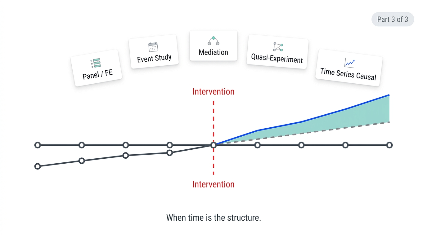
Part 3 of 3 — Longitudinal estimation, pathway analysis, natural experiments, and causal inference when your data has a time dimension that matters.
Parts 1 and 2 covered the core quasi-experimental methods and the modern ML-enhanced causal toolkit. This final part covers the methods that operate on the time dimension of data — leveraging the structure of panels, the timing of events, and the dynamics of time series to extract causal estimates from data that would otherwise yield only correlations.
These methods are particularly relevant for business analytics because business data is almost always longitudinal. You have stores observed week over week. Customers observed transaction by transaction. Markets observed quarter by quarter. The temporal structure in that data is not just a feature engineering opportunity — it is a source of identifying variation that, used correctly, produces some of the most credible causal estimates available from observational data.
Method 9: Panel Data and Fixed Effects Estimation
The problem it solves: When you observe the same units (stores, customers, employees, products) across multiple time periods, you have a panel — and that panel contains a powerful natural control mechanism. Each unit serves as its own control across time. Fixed effects estimation exploits this structure to eliminate all time-invariant confounders in one shot, without having to observe or measure them.
The core idea: A unit fixed effect absorbs everything about a unit that doesn't change over time — its location, its historical culture, its management team's baseline competence, its customer demographics. A time fixed effect absorbs everything that was happening in the world during a given period — macroeconomic shocks, category trends, seasonal patterns. With both sets of fixed effects included, the identifying variation comes entirely from within-unit changes over time, after removing universal time trends.
Within-unit variation is the identifying mechanism. The coefficient on the treatment variable is estimated from changes within the same store over time, not from differences between stores. If Store A received the treatment in week 20 and Store B never did, the fixed effects model asks: how did Store A's outcome change from its own pre-treatment baseline, relative to how Store B changed over the same period? The within-unit comparison removes all stable differences between stores — no need to observe or measure them.
The limitation: Fixed effects cannot control for time-varying confounders — factors that are changing differently across units over time and also affect the outcome. If stores that received treatment were simultaneously undertaking other improvements that the control stores were not, fixed effects will attribute those improvements to the treatment. This is the residual threat to identification after fixed effects are applied, and it requires theoretical argumentation rather than statistical resolution.
Best business applications: Store-level operations analysis, customer behavior over lifecycle stages, employee performance across tenure, product performance across markets — any setting with repeated observations of the same units over time.
Method 10: Event Study Design
The problem it solves: DiD with two time periods (pre and post) estimates a single treatment effect. Event study design extends this to multiple time periods, estimating treatment effects for each period relative to the treatment date. This serves two functions simultaneously: it validates the parallel trends assumption by examining pre-treatment dynamics, and it characterizes the treatment effect's evolution over time — immediate shock, gradual ramp-up, or decay.
The mechanics: Estimate a regression with interactions between the treatment indicator and period-relative-to-treatment dummies. Period -1 (the period just before treatment) is the omitted reference category.
Reading the event study plot: Pre-treatment coefficients (periods -8 through -1) should be statistically indistinguishable from zero. If they're not — if there's a pre-trend visible in the data — the parallel trends assumption fails and the DiD estimate is invalid. A well-specified event study plot with flat pre-treatment coefficients is the gold-standard diagnostic for DiD validity.
Post-treatment coefficients reveal the treatment effect's dynamics. An immediate jump at period 0 that persists flat suggests a permanent level shift. A gradual ramp from period 0 to period +4 suggests diffusion. A spike at period 0 that decays toward zero suggests a novelty effect with no lasting impact.
Best business applications: Policy or program evaluation where treatment timing varies across units (staggered adoption). New product launches where the ramp-up profile matters for demand forecasting. Organizational changes where the speed of impact is as important as the magnitude.

Method 11: Mediation Analysis
The problem it solves: Most causal analysis asks whether X causes Y. Mediation analysis asks how — through what pathway does X affect Y? This matters enormously when the treatment has multiple downstream mechanisms and you want to understand which ones to invest in, amplify, or block.
The conceptual framework: The total effect of X on Y decomposes into a direct effect (X → Y, not through the mediator) and an indirect effect (X → M → Y, running through the mediating variable M). Separating these requires a structural model of the causal pathway.
Total Effect = Direct Effect + Indirect Effect
TE = DE + IE
Where:
IE = (effect of X on M) × (effect of M on Y, controlling for X)
The critical assumption: The mediator M must not be confounded with the outcome Y — there must be no unmeasured common causes of M and Y. This is called the sequential ignorability assumption, and it is demanding. In practice, mediation analysis provides its most credible estimates when the mediator itself was randomized (as in some two-stage experimental designs) or when the causal pathway is well-supported by domain knowledge.
Best business applications: Evaluating whether a price change affects revenue directly or primarily through changing customer acquisition rates. Understanding whether a training program improves sales performance through skill development (direct) or through confidence and motivation (indirect, through engagement). Decomposing customer retention into direct loyalty program effects and indirect network effects.
Method 12: Quasi-Experiments — The Natural Experiment Mindset
The problem it solves: Sometimes nature, policy, or business operations generate variation in treatment that is as good as random — not because anyone designed an experiment, but because the assignment mechanism was driven by factors unrelated to the outcome.
The core idea: A natural experiment is any setting where external circumstances — a law change, a lottery, a supply shock, a geographic boundary, a weather event — create a source of variation in treatment that is plausibly exogenous to the outcome. Finding and exploiting these natural experiments is as much a mindset as a method.
Common natural experiment structures in business:
Geographic discontinuities: Regulatory differences across state or country borders create natural variation in exposure to policies. Stores on one side of a border face different minimum wage laws, tax rates, or advertising regulations. The geographic boundary is the source of exogenous variation.
Supply shocks: A supplier disruption that randomly affects some product categories but not others creates exogenous variation in availability. Which categories experienced the shock is driven by logistics, not by category performance.
Lottery and random allocation: Any internal business process that randomly allocates resources — randomized customer service agent assignment, randomized order in which customers are contacted, randomized order of serving queues — generates natural experimental variation that can be analyzed with standard methods.
Timing variation from operational constraints: When a program is rolled out sequentially to units due to operational capacity constraints, and the ordering of rollout was not determined by unit performance, the rollout order creates a natural waitlist control group.
Method 13: Time Series Causal Methods
The problem it solves: When data has a strong temporal structure — where past values of a variable influence future values, and where multiple series co-evolve over time — standard cross-sectional causal methods are insufficient. Time series causal methods use the temporal ordering of events to extract causal information.
Granger Causality is the foundational time series causality test. Variable X "Granger causes" Y if past values of X help predict future values of Y beyond what Y's own past values predict. It is important to understand what this is and is not: Granger causality is predictive causality, not structural causality. It identifies useful predictive relationships in time-ordered data, not necessarily the causal mechanisms behind them.
Best business applications of time series causal methods: Evaluating the impact of a marketing campaign on a brand's sales trajectory. Assessing whether a pricing change permanently shifted a category's growth rate. Measuring the effect of an operational process change on a supply chain metric. Any context where a single time series captures the outcome and the intervention date is known.
The Complete Econometrics Toolkit — A Reference Summary
Across all three parts of this series, the complete toolkit covers thirteen methods organized by their data requirements and identifying assumptions:
Cross-sectional methods with strong assumptions
- Propensity Score Matching — requires unconfoundedness on observables
Panel / longitudinal methods
- Difference-in-Differences — requires parallel trends
- Two-Way Fixed Effects — eliminates time-invariant confounders
- Event Study Design — validates parallel trends, characterizes effect dynamics
- Synthetic Control — requires pre-treatment fit quality in donor pool
Threshold and discontinuity methods
- Regression Discontinuity Design — requires no manipulation at threshold
Instrumental methods
- Instrumental Variables — requires exclusion restriction
Experimental and semi-experimental methods
- A/B Testing — requires successful randomization
- Natural / Quasi-Experiments — requires exogenous source of treatment variation
Effect heterogeneity methods
- Uplift Modeling — requires experimental training data or unconfoundedness
- Causal Forests — requires experimental data or unconfoundedness, provides valid CI
Pathway methods
- Mediation Analysis — requires sequential ignorability
Time series methods
- Granger Causality — predictive causality in time-ordered data
- Interrupted Time Series — requires stable pre-intervention trend
What Makes a Causal Analyst
Reading this series is the beginning of building a causal toolkit, not the end. The methods are learnable. The harder skill — the one that makes a data scientist genuinely dangerous in the good sense — is the judgment to know which method fits which problem, which assumptions are credible in a specific business context, and how to explain those assumptions to a stakeholder who didn't study econometrics.
Causal analysis is ultimately an argument. The methods provide the structure of the argument. The domain knowledge and intellectual honesty of the analyst determine whether the argument is convincing and whether the conclusions drawn from it can be trusted.
That combination — rigorous method, honest assumption assessment, and clear communication — is what separates analysis that drives decisions from analysis that fills slide decks.
This post is part of DSBootcamp's Econometrics series, where we cover the causal inference methods and statistical frameworks that separate credible business analysis from expensive guesswork.