Smarter Replenishment: Demand Forecasting for Finished Goods Using Moving Average & Exponential Smoothing
Your shelves are empty — but your warehouse report said otherwise.
Problem Statement
CrestBridge Distribution Co. is a regional fast-moving consumer goods (FMCG) distributor headquartered in Atlanta, serving retail chains, grocery stores, and e-commerce fulfilment centers across the southeastern United States. Over the past two years, CrestBridge has managed a portfolio of 40 finished goods SKUs spanning four product categories — Beverages, Snack Foods, Personal Care, and Household Products — distributed out of six regional warehouses.
Despite steady overall revenue growth, the operations planning team has flagged a recurring and costly problem: demand-supply mismatches are causing stockouts and overstock situations simultaneously across different SKUs. In Q3 2024 alone, the company reported $480,000 in lost sales from stockouts on high-velocity Beverage SKUs, while simultaneously writing off $210,000 in excess Household Products inventory that had accumulated beyond shelf life. Root cause analysis pointed to a single gap — the replenishment team was still relying on a simple "last month's sales" heuristic to set next month's purchase orders, with no systematic method to account for trend or seasonality.
You have been brought in as a Data Analyst for a two-week project to build CrestBridge's first data-driven demand forecasting baseline. Using two years of weekly sales order data (January 2023 – December 2024, approximately 12,000 transactions), your task is to aggregate historical demand at the weekly level per product category, apply Simple Moving Average (SMA) and Single Exponential Smoothing (SES) forecasting methods, visualize actual versus forecast demand, and evaluate both methods using MAE and RMSE. The output will directly inform the replenishment team's monthly purchase order quantities for Q1 2025 — replacing the last-month heuristic with a defensible, repeatable analytical approach.
Stakeholder Requirements
--Aggregate raw sales order data into a clean weekly demand time series per product category (after resolving data quality issues), and produce a line chart showing the demand trend and seasonality patterns across all four categories for the full 2023–2024 period.
--Apply Simple Moving Average (4-week window) and Single Exponential Smoothing (α = 0.3) to the weekly demand series for each product category. Plot actual vs. both forecast lines on the same chart and calculate MAE and RMSE for each method per category.
--Based on forecast error comparison, select the better-performing method per category and use its final forecast value to recommend a replenishment quantity for the first week of Q1 2025 for each category, presented as a structured summary table.
Domain Understanding
FMCG Distribution & Demand Planning Overview
In FMCG distribution, finished goods are products that have completed the manufacturing process and are ready for sale to end customers — beverages, packaged foods, personal care items, and household products. Distributors like CrestBridge sit between manufacturers and retailers, holding inventory in regional warehouses and fulfilling purchase orders as retail demand materialises. The core planning challenge is that distributors must commit to replenishment orders weeks in advance (to account for supplier lead times of 2–6 weeks), while actual retail demand only becomes visible at point of sale. This lag between commitment and observation is what makes demand forecasting critical. Without a systematic forecast, planners either over-order (creating holding costs, spoilage risk, and working capital strain) or under-order (creating stockouts, lost sales, and retailer relationship damage). The fundamental goal of demand forecasting in this context is not to predict the future perfectly — it is to reduce the cost of being wrong.
Critical Metrics & Calculations
Five metrics define the forecasting and replenishment domain:
1. Weekly Demand (Units)
Weekly Demand = Sum of quantity_fulfilled for all orders in a given week
The foundational time series input. Note that quantity_fulfilled (not quantity_ordered) reflects actual demand met — a better proxy for true market demand, though it understates demand when stockouts occur.
2. Simple Moving Average (SMA)
SMA(t, n) = (D(t-1) + D(t-2) + ... + D(t-n)) / n
where D(t) is demand in week t and n is the window size. SMA smooths out short-term noise by averaging the last n periods. A 4-week window is common in weekly FMCG planning — long enough to smooth noise, short enough to stay responsive to trend shifts.
3. Single Exponential Smoothing (SES)
SES(t) = α × D(t-1) + (1 - α) × SES(t-1)
where α (alpha) is the smoothing factor between 0 and 1. Higher α makes the forecast more responsive to recent demand; lower α gives more weight to historical patterns. α = 0.3 is a widely used starting point for stable-demand products.
4. Mean Absolute Error (MAE)
MAE = Mean(|Actual(t) - Forecast(t)|)
Measures the average magnitude of forecast error in the same units as demand (units/week). Easy to interpret: an MAE of 200 means forecasts are off by 200 units per week on average.
5. Root Mean Squared Error (RMSE)
RMSE = sqrt(Mean((Actual(t) - Forecast(t))²))
Penalises large errors more heavily than MAE. An RMSE significantly higher than MAE indicates the model occasionally makes very large errors — a red flag for a replenishment system where a single large miss can cause a stockout.
Business Logic & Trade-offs
The choice between SMA and SES involves a real trade-off that practitioners must understand. SMA treats all n historical periods equally — it is simple, transparent, and easy to explain to non-technical stakeholders. SES, by contrast, gives exponentially more weight to recent demand, making it faster to respond when demand is shifting (e.g., a product gaining popularity or declining). For stable, seasonally predictable categories like Household Products, SMA often performs comparably to SES. For categories with irregular demand shifts or promotions — like Beverages in summer — SES tends to track actual demand more closely because it reacts faster to the upturn.
One important practical constraint: both SMA and SES produce a one-step-ahead forecast (next week's demand based on past weeks). For replenishment planning with a 4–6 week lead time, planners typically apply the same forecast value forward across the lead time window, which amplifies any systematic bias. This is why even small reductions in MAE translate to meaningful inventory improvements at scale. A second constraint to keep in mind: neither SMA nor SES captures seasonality explicitly — a Beverage category with a clear summer peak will produce forecasts that perpetually lag the seasonal upturn when using these baseline methods. Identifying that limitation in the data is itself a valuable analytical output, and a natural motivation for more advanced methods (Holt-Winters, SARIMA) in future iterations.
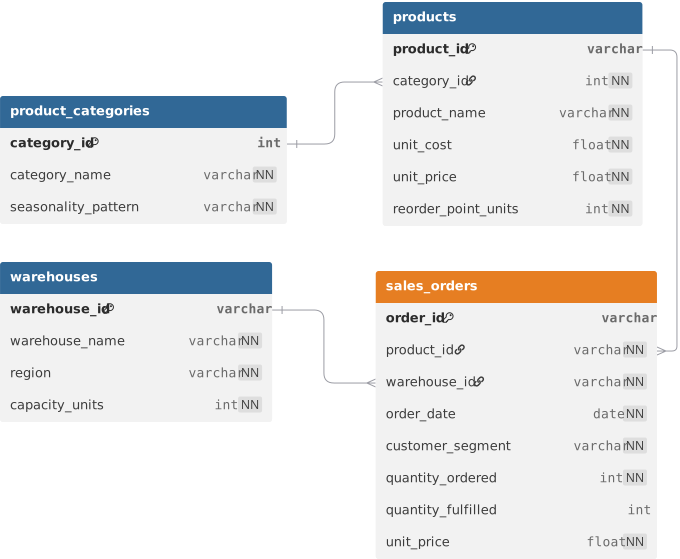
ER Diagram
Loading the interactive workspace...