Maximize Listing Revenue: Dynamic Price Optimization

PriceWave is a mid-sized online marketplace platform headquartered in Austin, Texas, hosting over 6,000 active product listings across five major categories: Electronics, Home & Kitchen, Apparel, Sports & Outdoors, and Beauty & Personal Care. Between January 2022 and December 2025, PriceWave processed approximately 19,000 individual listing-pricing events — moments when a seller either set a new price, the platform refreshed a price recommendation, or a listing went live with a competitive price position. Despite consistent platform growth of 17% year-over-year in gross merchandise value (GMV), PriceWave's analytics team has flagged a troubling pattern: a significant share of listings are systematically underpricing or overpricing relative to competitor benchmarks. Underpriced listings sacrifice margin and trigger race-to-the-bottom dynamics; overpriced listings sit unsold, degrading conversion rates and seller satisfaction scores.

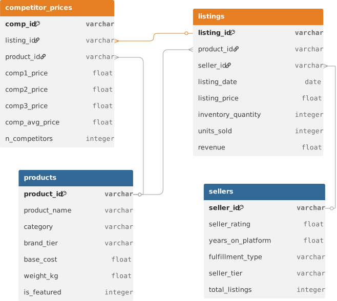
The Director of Marketplace Analytics, Priya Anand, has commissioned a demand-based dynamic pricing study. The core hypothesis is that units sold on any given listing is a function of several controllable and observable variables — most importantly the ratio of the listing's price to the competitor average price, but also product category, seller performance metrics, inventory levels, and seasonality. By building a regression model that quantifies how demand responds to these inputs, PriceWave can estimate price elasticity for each product category and use it to compute a revenue-maximizing price for any listing at any point in time. As the data analyst on this project, you will merge listing data, competitor price benchmarks, and seller performance metrics into a single analytical dataset, engineer key pricing features (price ratio, price gap, competitive position), fit a Multiple Linear Regression model predicting units sold, derive category-level price elasticities from the model's coefficients, and finally build a dynamic pricing recommendation engine that outputs an optimal price for any listing given current competitor prices and inventory conditions. Your output will directly feed PriceWave's automated repricing system launching next quarter.

--Build a Multiple Linear Regression model predicting units_sold using engineered pricing features (price ratio vs. competitors, price gap, competitive position rank), seller performance metrics, product category (one-hot encoded), and seasonal indicators; report model performance using R², RMSE, and MAE on a held-out test set, and verify the model outperforms a baseline that predicts the mean units sold for all listings.

--Derive and visualize category-level price elasticity estimates from the model's coefficients — compute the elasticity for each of the five product categories and interpret which categories are most and least price-sensitive, explaining the business implication in plain language suitable for Priya Anand's team.

--Build a dynamic pricing recommendation function that accepts a listing's product category, seller rating, current inventory level, and a set of competitor prices as inputs, and returns the revenue-maximizing optimal price using the fitted regression model; demonstrate the function on five representative listing scenarios across different categories and report the recommended price alongside the estimated units sold at that price.

Dynamic Pricing and Marketplace Economics

Dynamic pricing is the practice of adjusting product prices in real time based on market signals — competitor prices, demand patterns, inventory levels, and buyer behavior. In marketplace platforms (Amazon, eBay, Etsy, and mid-tier platforms like PriceWave), pricing is particularly complex because sellers compete simultaneously on price, seller reputation, fulfillment speed, and listing quality. The platform itself has a layered incentive: it wants sellers to achieve high conversion rates (generating GMV-based take rate revenue), but also wants to prevent destructive price wars that commoditize listings and erode seller loyalty. Analysts working on dynamic pricing problems must understand that the price a seller sets is not the only variable a buyer sees — they see a price relative to alternatives. This is why competitive price benchmarking is the foundational data requirement: you cannot model demand without knowing where a listing sits in the competitive landscape. In practice, competitive price data is scraped or API-sourced from competitors at regular intervals, creating a panel dataset of price positions over time.

Critical Metrics & Calculations

Five metrics drive dynamic pricing analytics and elasticity modeling:

Price Ratio: Price Ratio = Our Price / Competitor Average Price. A ratio of 1.0 means price parity; below 1.0 means we are cheaper than the market; above 1.0 means we are more expensive. This is the single most important feature in demand modeling — it captures competitive positioning better than absolute price alone because it accounts for market-level price movement over time.

Price Elasticity of Demand: ε = (% Change in Quantity Demanded) / (% Change in Price). For most consumer goods, elasticity is negative (higher price → lower demand). A value of −2.0 means a 1% price increase causes a 2% drop in units sold. Electronics typically have elasticity of −2.0 to −3.5; staple household goods are around −0.8 to −1.5; luxury or brand-driven goods can be near −0.5. In a regression context, if the coefficient on log(price) in a log(units) model is −1.8, that is the elasticity estimate directly.

Revenue-Maximizing Price: For a linear demand curve Q = a − b × P, revenue R = P × Q = aP − bP². Taking dR/dP = 0: P* = a / (2b). In practice with regression outputs, this becomes an iterative search over a price grid to find the price that maximizes P × predicted_Q(P).

Competitive Price Position: Rank among N competitors + 1 (1 = cheapest, N+1 = most expensive). A listing ranked 1st among 4 competitors is the price leader; ranked 4th is the most expensive. This ordinal feature captures relative positioning effects that the continuous price ratio misses.

Conversion Rate Proxy: Units Sold / Listing Views when view data is available; when not, Units Sold per listing period is used as a demand proxy. PriceWave uses units sold per 30-day listing window as its primary demand signal.

Business Logic & Trade-offs

The central tension in dynamic pricing is between margin optimization and volume maximization. Cutting price to gain market share works until competitors retaliate, collapsing the price floor for the entire category — a pattern well-documented in electronics and commodity household goods. Holding price high preserves margin but risks losing the sale entirely if buyer search cost is low (as it is on any marketplace with visible competitor listings). The regression model you build here estimates where a listing currently sits on its demand curve; the revenue-maximizing price formula then finds the price point where the marginal gain in price is exactly offset by the marginal loss in volume.

A critical modeling consideration at difficulty 4 is multicollinearity between price features. our_price, comp_avg_price, price_ratio, and price_gap are all mathematically related. Including all of them in a regression simultaneously creates severe multicollinearity — inflating standard errors and making coefficients unstable. The correct approach is to select the most informative representation: price_ratio and price_gap together capture the competitive dimension cleanly without the redundancy of including raw prices alongside them. A second consideration is heteroscedasticity in demand data: listings with high average demand (electronics, popular apparel) have much more variable unit counts than niche listings, violating the constant-variance assumption of OLS. Checking a residuals plot is a necessary validation step at this difficulty level. Finally, be aware that seasonal demand spikes (Q4 holiday, back-to-school) are confounders — a listing that happened to run during December will show higher units sold regardless of its price position, which is why month and quarter indicators must be included as controls.