
Most business experiments are designed to detect effects they were never powered to find. Here's the sample size math and why this matters more than any other experimental design decision.
A product team runs a two-week A/B test on a new checkout flow. Results come back: the treatment group shows a 1.8% lift in conversion rate. The p-value is 0.21. The conclusion written in the experiment summary: "No significant effect detected. Rolling back."
Here is what almost certainly happened instead: the test was underpowered. It was never capable of detecting a 1.8% lift with any reliability. If the true effect was real, the test would have missed it roughly 70% of the time regardless of the data collected. The rollback decision wasn't based on evidence that the feature doesn't work. It was based on the absence of evidence — and the absence was manufactured by a flawed experimental design made before a single user was exposed.
Underpowered experiments are not edge cases. They are the default in most business experimentation programs, and they produce a specific, costly pattern: real product improvements get abandoned, ineffective changes get falsely validated when noise briefly tips a test positive, and teams lose confidence in experimentation as a decision-making tool. All of this is preventable with math that takes ten minutes to run before the test starts.
The Four Numbers That Govern Every Experiment
Statistical power is determined by four inputs, and understanding their relationship is the entire foundation of experiment design. Every decision you make about an experiment either explicitly or implicitly sets values for these four numbers:
Significance level (α): The probability of a false positive — concluding there's an effect when there isn't one. The conventional default is 0.05. This means you accept a 5% chance of declaring a winner when the null hypothesis is actually true.
Statistical power (1 - β): The probability of detecting a true effect when one exists. The conventional target is 0.80 — meaning an 80% chance of finding the effect if it's real. Equivalently, β = 0.20 is the false negative rate you're accepting. Most underpowered tests are running at 0.40 or 0.50 power without knowing it.
Minimum Detectable Effect (MDE): The smallest true effect size you want the experiment to reliably detect. This is the most important and most frequently misspecified input. Setting a realistic MDE requires a business judgment about what effect size would actually matter — not the effect you hope to see.
Baseline metric and variance: The current conversion rate, mean, or proportion you're measuring against, along with an estimate of its variability.
These four numbers are bound by a formula — change any one and the others must adjust. The most common mistake in experiment design is specifying α, assuming 80% power, guessing an optimistic MDE, and never computing the required sample size until after the test runs and fails to reach significance.
The Sample Size Formula
For a two-proportion test — the most common case in business experimentation (conversion rates, click rates, activation rates) — the required sample size per group is:
n = 2 × (Z_α/2 + Z_β)² × p(1 - p) / MDE²
Where:
- Z_α/2 = 1.96 for α = 0.05 (two-tailed)
- Z_β = 0.84 for 80% power (β = 0.20)
- p = baseline conversion rate
- MDE = minimum detectable effect as an absolute difference
The combined Z-score constant (1.96 + 0.84)² = 7.84 is worth memorizing — it's the core multiplier for the standard experimental design.
Run this below before every experiment. It takes thirty seconds and prevents the category of mistake that opens this post.
import numpy as np
from scipy import stats

def sample_size_per_group(
    baseline_rate: float,
    mde: float,
    alpha: float = 0.05,
    power: float = 0.80
) -> int:
    """
    Compute required sample size per group for a two-proportion z-test.

    Parameters
    ----------
    baseline_rate : float  — current conversion rate (e.g., 0.12 for 12%)
    mde           : float  — minimum detectable effect, absolute (e.g., 0.02)
    alpha         : float  — significance level (default 0.05)
    power         : float  — desired power (default 0.80)

    Returns
    -------
    int — sample size required per group
    """
    z_alpha = stats.norm.ppf(1 - alpha / 2)
    z_beta  = stats.norm.ppf(power)

    p1 = baseline_rate
    p2 = baseline_rate + mde
    p_bar = (p1 + p2) / 2

    n = (2 * p_bar * (1 - p_bar) * (z_alpha + z_beta) ** 2) / (mde ** 2)
    return int(np.ceil(n))


# Example: checkout conversion rate = 4.5%, want to detect a 0.5pp lift
n = sample_size_per_group(baseline_rate=0.045, mde=0.005)
print(f"Required sample size per group: {n:,}")
print(f"Total experiment size: {2 * n:,}")
Why MDE Is the Decision That Actually Matters
The MDE is the input that teams consistently get wrong — almost always by setting it too high, which dramatically reduces the required sample size and makes the test appear feasible when it isn't.
The logic failure goes like this: a team wants to run a quick test, so they set the MDE at 5 percentage points to make the required sample size manageable. But the realistic business effect of the change they're testing is probably 0.5 to 1.5 percentage points. The test is designed to detect effects three to ten times larger than reality. It will almost certainly return a null result — not because the feature doesn't work, but because the experiment was designed to be blind to the magnitude of effects that would actually occur.
The right way to set the MDE is backward from business impact. Ask: what is the smallest effect size that would make this change worth shipping? Factor in the development cost, the opportunity cost of the engineering time, the maintenance burden, and the revenue impact of the effect. If a 0.3% lift in checkout conversion generates $200,000 per year in revenue and the cost of shipping the feature is $50,000, a 0.3% lift is worth detecting. Set the MDE at 0.003 — and if the required sample size is larger than your current traffic supports, acknowledge that directly rather than inflating the MDE until the math is convenient.
# MDE sensitivity table — what effect sizes can you detect at current traffic?
import pandas as pd

weekly_traffic = 5000       # users per week per group
available_weeks = 2         # test duration you have
n_available = weekly_traffic * available_weeks

baseline = 0.045
results = []

for mde_pp in [0.001, 0.002, 0.005, 0.010, 0.015, 0.020]:
    n_required = sample_size_per_group(baseline, mde_pp)
    feasible = n_available >= n_required
    weeks_needed = np.ceil(n_required / weekly_traffic)
    results.append({
        'MDE (pp)': f"{mde_pp*100:.1f}%",
        'n Required': f"{n_required:,}",
        'Weeks Needed': int(weeks_needed),
        'Feasible in 2 Weeks': '✓' if feasible else '✗'
    })
This table is the artifact that resets the team's expectations. When everyone can see that detecting a 0.5% lift requires 14 weeks of traffic and they only have 2, the conversation shifts to the right questions: should we run a longer test, should we find a more sensitive metric, or should we accept that this effect size is below our current experimental resolution and make the decision on business logic alone?
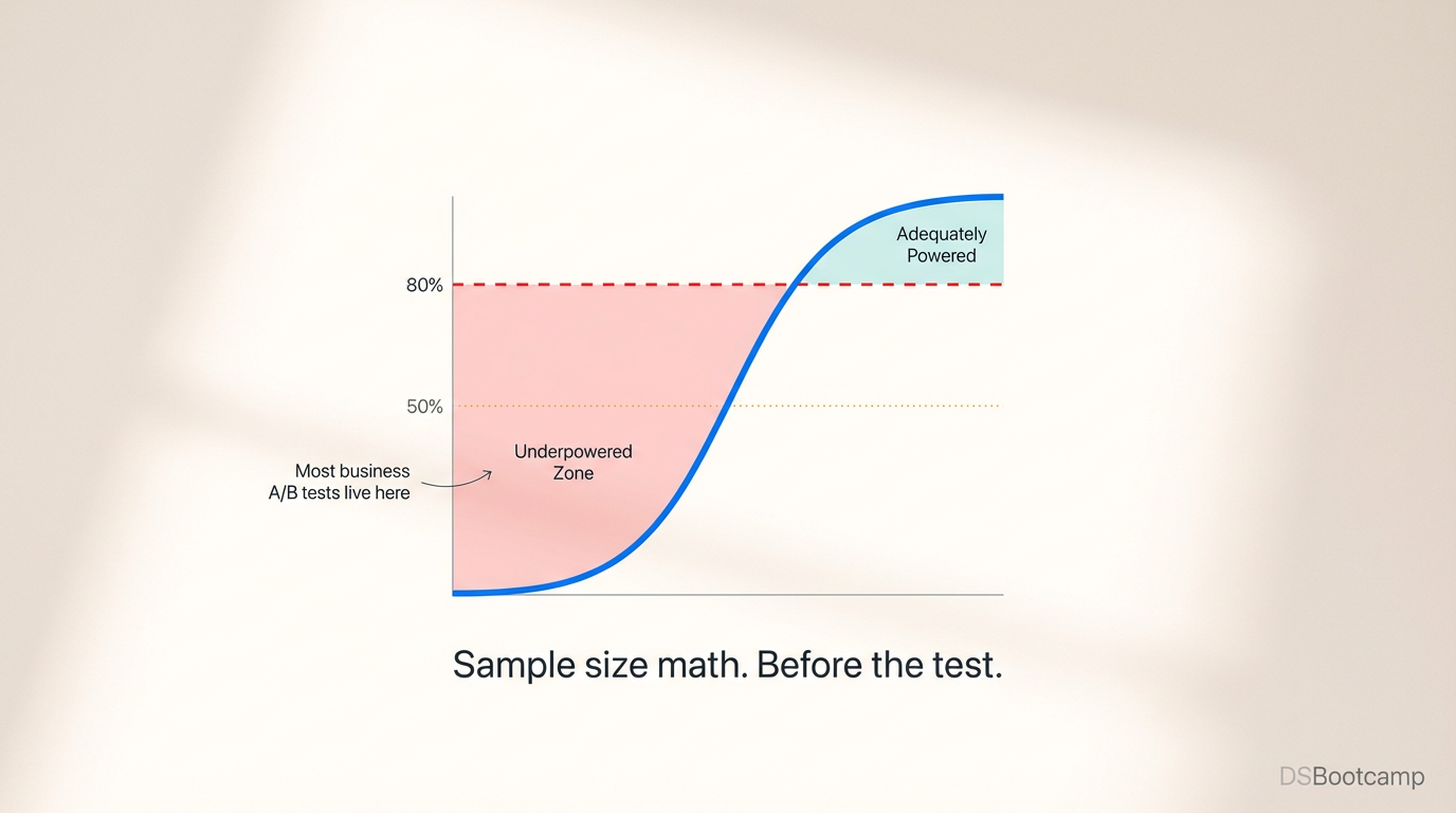
The Power Curve: Reading Your Experiment's Actual Capability
A single sample size calculation tells you whether your experiment is powered for one specific MDE. A power curve shows you the full range — what your experiment can and cannot detect across all effect sizes.
import matplotlib.pyplot as plt
from statsmodels.stats.power import NormalIndPower

analysis = NormalIndPower()

effect_sizes = np.linspace(0.001, 0.030, 100)
powers = []

for mde in effect_sizes:
    # Convert to Cohen's h for proportions
    p2 = baseline + mde
    from statsmodels.stats.proportion import proportion_effectsize
    h = abs(proportion_effectsize(baseline, p2))
    pwr = analysis.power(effect_size=h, nobs1=n_available, alpha=0.05)
    powers.append(pwr)

plt.figure(figsize=(8, 5))
plt.plot(np.array(effect_sizes) * 100, powers, color='steelblue', lw=2)
plt.axhline(0.80, color='red', linestyle='--', label='80% Power threshold')
plt.axhline(0.50, color='orange', linestyle=':', label='50% Power (coin flip)')
plt.xlabel('True Effect Size (percentage points)')
plt.ylabel('Statistical Power')
plt.title(f'Power Curve — n={n_available:,} per group, baseline={baseline*100}%')
plt.legend()
plt.grid(alpha=0.3)
plt.tight_layout()
plt.show()
The power curve delivers a fact that no stakeholder can argue with: "At our current traffic levels over a two-week test, we have 80% power to detect effects of 1.2 percentage points or larger. Effects smaller than that are in the grey zone — we may or may not detect them. Before we start, we should agree: if the result comes back null, it means we didn't detect an effect at or above 1.2pp. It does not mean the feature has no effect."
Setting that expectation before the test runs is the difference between a null result that drives a clear decision and a null result that generates two weeks of argument about whether the test was valid.
Common Traps That Underpower Tests in Practice
Stopping early when results look good. Peeking at results and stopping when p < 0.05 is reached inflates the false positive rate dramatically. The sample size calculation assumes you will collect the pre-specified number of observations. Stopping at 60% of the required sample because the early numbers look promising is a guarantee of underpowered, unreliable results. Use sequential testing methods (like the always-valid p-value or SPRT) if you genuinely need the option to stop early.
Using traffic instead of users. If the same user can appear in your experiment data multiple times (multiple sessions, multiple page views), you cannot treat each row as an independent observation. The effective sample size is the number of unique users, not the number of events. Calculating power on event counts when the unit of randomization is users will make your test appear vastly better powered than it is.
Ignoring metric variance. For continuous metrics (revenue per user, session duration, order value), variance dominates the sample size calculation more than baseline level. High-variance metrics require dramatically larger samples than low-variance ones. Always pull the actual standard deviation from historical data rather than estimating it.
Running too many variants. Adding a third or fourth variant doesn't double your statistical burden — it multiplies it. A test with four variants (one control, three treatments) requires correcting for multiple comparisons, which pushes the effective α threshold down and requires more observations per group to maintain power. Every variant you add should be justified by a specific, distinct hypothesis — not by curiosity.
The Pre-Experiment Checklist
Before launching any experiment:
Seven checks. Running an experiment without them isn't faster — it just defers the cost to the analysis phase, where an underpowered null result requires relitigating the entire design from scratch.
The math is not the hard part. The discipline to run it before the test starts, and to accept what it tells you when the required sample is larger than convenient, is where most experimentation programs fail. That discipline is exactly what separates teams that learn from experiments from teams that argue about them.
This post is part of DSBootcamp's Econometrics series, where we cover the experimental design, causal inference, and statistical frameworks that make business analysis credible and actionable.