
Most data science courses teach you how to work with data. What they rarely teach you is which kind of data you'll actually be staring at on a Monday morning when a pipeline breaks or a stakeholder asks why the model started behaving differently last week.
The truth is that "data" in production is not a single thing. It's a family of very different animals, each with its own structure, storage patterns, failure modes, and analytical techniques. Treating them as interchangeable is one of the fastest ways to build systems that look fine in notebooks and fall apart in the real world.
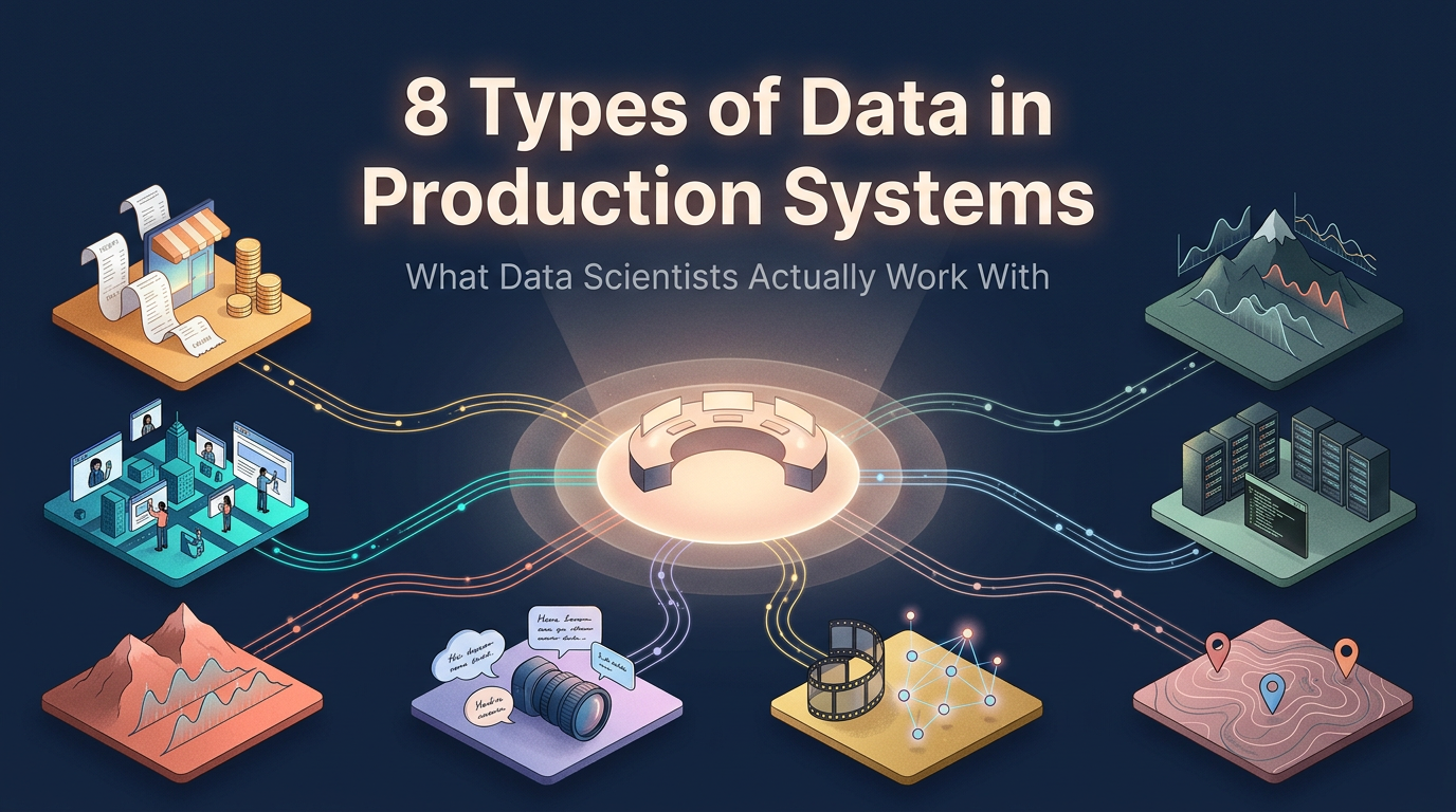
This article walks through the 8 types of data that data scientists and analysts most commonly encounter in real-world production systems: what each type looks like, where it comes from, and what you need to watch out for.
1. Transactional Data
If there's one type of data that keeps business analysts employed, it's transactional data. Every purchase made, every sign-up completed, every payment processed, every item added to a cart gets recorded as a transaction. This is the foundational layer of most business intelligence work.
Transactional data lives in relational databases like PostgreSQL, MySQL, Oracle, and Snowflake, organized into rows and columns with foreign keys stitching tables together. A single "transaction" in a retail system might span a dozen tables: the order header, the order lines, the customer record, the product catalog, the discount applied, the payment method used, and the shipment record.
On the surface, transactional data feels clean. It has schemas. It has constraints. It has audit logs. But in practice, it accumulates years of technical debt: tables designed for a business model that no longer exists, columns with ambiguous names, soft deletes that make WHERE active = 1 filters a landmine, and timezone handling that is almost always wrong somewhere.
What to watch for: Slowly Changing Dimensions (SCDs). Think about the customer who changed their address, the product whose category was reassigned, or the pricing rule that changed mid-quarter. Analysts who ignore this end up with attribution errors that are nearly impossible to trace.
2. Behavioral / Event Data
Where transactional data captures what happened at the business level, behavioral data captures what the user did at a granular, moment-by-moment level. Every page view, every button click, every scroll depth, every session start, every feature interaction are events, and in modern digital products, they are tracked obsessively.
This data typically flows through event tracking platforms like Segment, Mixpanel, Amplitude, or custom-built Kafka pipelines. The raw format is usually JSON or Avro, and events arrive in near real-time into a data warehouse like BigQuery or Redshift, where they are partitioned by date and event type.
Behavioral data is extraordinarily rich for product analytics, funnel analysis, retention modeling, and personalization. It's also extraordinarily expensive to work with at scale. A mid-sized SaaS product might generate hundreds of millions of events per day. Querying it naively, without partition pruning or pre-aggregation, will drain your compute budget and your patience simultaneously.
What to watch for: Event schema drift. Teams add new events, rename properties, or change data types without versioning or announcements. A user_id field that was a string in Q1 becomes an integer in Q3. Your joins break silently. Always validate event schemas before building pipelines on top of raw event tables.
3. Time Series Data
Time series data is any measurement recorded sequentially over time: stock prices sampled every second, server CPU utilization logged every minute, temperature readings from an IoT sensor every hour, weekly revenue figures every Monday. What defines it is not just the timestamp, but the fact that the order and spacing of observations carries meaning.
This type of data is common in finance, operations, infrastructure monitoring, manufacturing, energy, and healthcare. It arrives from sources as varied as Bloomberg terminals, Prometheus metrics exporters, SCADA systems, and wearable devices.
Working with time series data requires thinking differently from tabular analytics. You need to handle irregular sampling intervals, missing values caused by sensor downtime or network gaps, and non-stationarity, which is the tendency of the statistical properties of the series like its mean, variance, and autocorrelation to change over time. A model trained on pre-COVID sales data and deployed in 2021 is a vivid example of why stationarity assumptions matter.
What to watch for: Seasonality and lag. Time series data almost always has patterns at multiple frequencies simultaneously: daily, weekly, monthly, and yearly. Models that fail to account for these will consistently underperform. The gap between "the model looks good on average" and "the model is catastrophically wrong at 9am every Monday" is a seasonality problem.
4. Log Data
Every application, every server, every microservice is constantly writing to log files. When a user logs in, there's a log entry. When a function throws an exception, there's a stack trace. When a database query takes too long, there's a slow query log. When a container restarts, there's a system event recorded somewhere.
Log data is arguably the most information-dense type of data in any production system and also the most underutilized. It tends to be high volume, semi-structured or unstructured, and stored in systems like Elasticsearch, Splunk, or Datadog that are optimized for search and monitoring rather than analytical querying.
The challenge with log data is that it was almost never designed with analysis in mind. Log formats vary across services, often within the same company. Timestamps may be in different timezones. Key fields like request IDs that would allow you to join log events into a coherent trace are sometimes missing or inconsistently formatted.
Despite this, log data is invaluable for root cause analysis, anomaly detection, infrastructure capacity planning, and understanding failure modes that no other data source can explain. When a model starts producing unexpected outputs, the answer is often sitting in the logs, if you know how to look.
What to watch for: Log verbosity settings. Many systems are configured to only write ERROR and WARN level logs in production to manage storage costs. This means that by the time you want to investigate an incident, the fine-grained DEBUG logs that would have answered your question were never written in the first place.
5. Text / NLP Data
Text is the data type that most people interact with every day but that data science teams historically underinvested in, at least until large language models changed the economics. Customer reviews, support tickets, survey open-ends, social media posts, contract documents, call transcripts, medical notes: all of this is text, and all of it contains signal that structured data simply cannot capture.
Text data is unstructured in the sense that it has no fixed schema, but that does not mean it is chaotic. It has linguistic structure, sentiment, intent, topics, named entities, and discourse patterns, all of which can be extracted and quantified with the right techniques. Sentiment analysis, topic modeling, named entity recognition, intent classification, and summarization are the bread-and-butter NLP tasks that appear again and again in production.
What has changed dramatically in recent years is the baseline quality achievable with relatively little effort. Pre-trained transformer models have raised the floor substantially. A fine-tuned BERT or a prompted GPT-4 can deliver production-quality intent classification in a fraction of the time it once took. The engineering challenge has shifted from "how do we build the model" to "how do we handle hallucinations, latency, and cost at scale."
What to watch for: Distribution mismatch between training data and production data. A sentiment model trained on Amazon product reviews will not perform well on enterprise software support tickets. The vocabulary, sentence structure, domain jargon, and even the emotional register are completely different. Always validate text models on data that looks like your actual production inputs.
6. Graph / Relational Data
Some of the most interesting problems in data science are fundamentally about relationships rather than individual entities. How do fraudulent accounts cluster together? How does influence propagate through a social network? Which products are so often purchased together that recommending one should surface the other? These are graph problems, and they require a different mental model than tabular analysis.
Graph data represents entities as nodes and relationships as edges. A social graph has users as nodes and friendships as edges. A transaction fraud graph has accounts and merchants as nodes, with financial transactions as edges. A knowledge graph in a recommendation system might connect users, products, categories, brands, and behavioral signals in a single interconnected structure.
Graph databases like Neo4j or Amazon Neptune are designed to traverse these relationships efficiently. Graph neural networks (GNNs) have emerged as a powerful technique for learning from graph-structured data, particularly for fraud detection, drug discovery, and recommendation systems where the relational structure carries as much signal as the node features themselves.
What to watch for: Graph size and traversal depth. Graphs grow non-linearly. A simple "friends of friends" query that returns 100 results for one user might return 10 million for another who is well-connected. Naive graph queries on production systems without depth limits or sampling strategies can bring databases to their knees.
7. Geospatial Data
Location is a dimension that enriches almost any analysis it touches. Where a customer lives relative to a store affects their purchase frequency. Where a delivery driver is at 2pm affects whether the package arrives today. Where a new restaurant opens relative to competitors affects its survival probability. Geospatial data, including coordinates, polygons, routes, catchment areas, and administrative boundaries, makes these questions answerable.
Geospatial data comes in two primary flavors: vector data, which covers points, lines, and polygons like a store location, a road network, or a census tract boundary, and raster data, which covers gridded values over a geographic surface like satellite imagery or weather model output. Both require specialized tools to work with. Python's geopandas, shapely, and folium libraries, along with PostGIS for spatial SQL queries, are the standard toolkit for most production geospatial work.
Industries that use geospatial data heavily include retail (site selection, trade area analysis), logistics and delivery (route optimization, last-mile planning), real estate (valuation modeling, demand forecasting), agriculture (crop monitoring, yield prediction), and government (urban planning, public health surveillance).
What to watch for: Coordinate reference systems (CRS). Geospatial data from different sources often uses different projections and coordinate systems. Joining two datasets without aligning their CRS will produce results that are geometrically nonsensical, where points that appear to be in the same location are actually thousands of kilometers apart. Always verify and reproject before any spatial join or distance calculation.
8. Image / Video Data
Computer vision has moved well beyond academic benchmarks and into an enormous range of industries. Quality inspection on manufacturing lines, medical image analysis for diagnostics, satellite imagery for agricultural monitoring, facial recognition for access control, video analytics for retail foot traffic: image and video data is now a serious production data type for companies that would not traditionally think of themselves as computer vision companies.
The scale and storage requirements of image and video data are fundamentally different from tabular or text data. A single high-resolution image can be several megabytes. An hour of video footage can be gigabytes. Storing, retrieving, and preprocessing this data requires object storage systems like AWS S3 or Google Cloud Storage, purpose-built data pipelines, and often GPU-accelerated preprocessing.
Model training on image data also surfaces unique challenges: class imbalance (defective products are rare by design), annotation cost (labeling images requires human expert time), and data augmentation (flipping, rotating, and cropping images to artificially expand training sets). In medical imaging specifically, regulatory constraints around data access and model validation add another layer of complexity.
What to watch for: Label quality. Image annotation is expensive and error-prone. A mislabeled training example in a fraud detection or medical diagnostic model is not just a noise problem, it is a risk problem. Investing in annotation tooling and inter-annotator agreement metrics is not optional in high-stakes computer vision applications.
Putting It All Together
The reason this taxonomy matters in practice is that each data type demands a different stack, a different set of assumptions, and a different set of failure modes. A data scientist who only knows how to work with clean transactional data will be lost the first time they're handed a folder of PDF invoices, a Kafka topic of clickstream events, or a graph of financial transactions to analyze for fraud.
Real production systems almost always involve multiple data types working together. A recommendation engine might combine behavioral event data (what the user clicked), transactional data (what they purchased), graph data (what similar users bought), and text data (product descriptions and reviews), all joined, transformed, and served through a feature pipeline that needs to handle schema drift, missing values, and distribution shift simultaneously.
The mental model to carry forward is this: know which type of data you're working with before you write a single line of code. Each type has its grain, its natural keys, its temporal properties, and its failure modes. Getting that foundation right is what separates analysts who build things that work in production from those who build things that work in notebooks.