
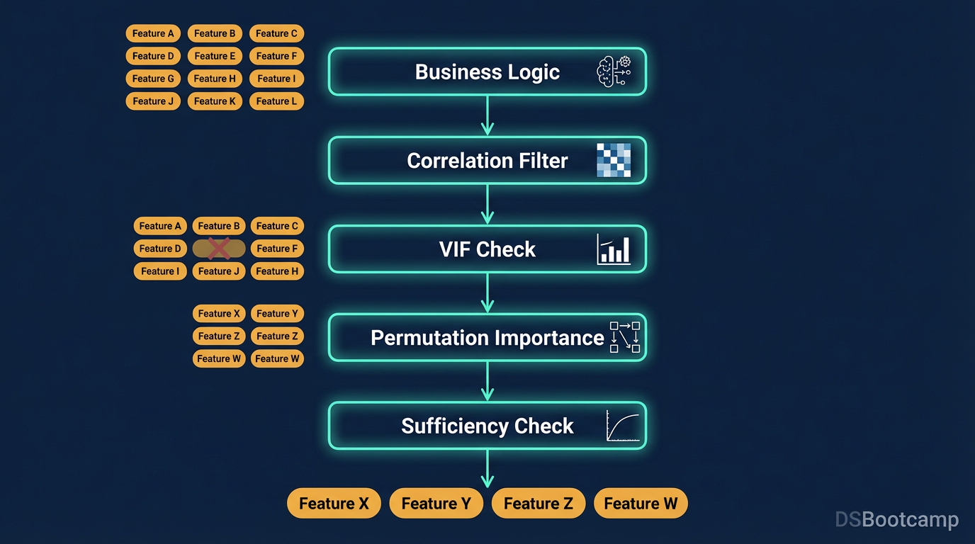
Start with business logic, filter by correlation, check VIF, run permutation importance, and know when enough features is enough.
Feature selection is where most data science tutorials skip straight to the code and most production models quietly go wrong. The pattern is familiar: a dataset arrives with 80 columns, the analyst drops a few obviously irrelevant ones, throws the rest into a random forest, and calls the feature importance plot a selection process. The model trains. The metrics look reasonable. The whole thing ships.
Six months later, the model degrades in production because three of those 80 features were subtly leaking future information, two more were so correlated they were destabilizing the coefficient estimates, and nobody ever asked whether the features that scored highest on importance actually made business sense.
Feature selection done properly is a five-stage process — not a single step. Each stage catches a different class of problem. Skipping any of them doesn't make your model wrong immediately; it makes it fragile in ways that only become visible later, usually in production, usually at the worst possible time.
This is the full process.
Stage 1: Business Logic Review — Before Any Code Runs
The first filter on your feature set should happen entirely away from a keyboard. Take the raw list of candidate features and ask three questions about each one.
Does this feature have a plausible causal or explanatory relationship with the target? Not correlation — causation or at least a defensible mechanism. If you're predicting customer churn, "days since last purchase" has an obvious mechanism. "Customer ID modulo 7" does not, even if it correlates in your training data. Features without a mechanism are noise masquerading as signal, and they will fail silently when the data distribution shifts.
Would this feature be available at prediction time in production? This is the data leakage question. It is surprisingly easy to include a feature that is only available after the event you're trying to predict. If you're predicting whether a transaction is fraudulent, the "refund requested" flag is not a feature — it's a consequence. Check the timestamp logic on every feature before it enters the pipeline.
Does including this feature raise any fairness or regulatory concerns? In credit, hiring, healthcare, or any regulated domain, features that are proxies for protected characteristics — zip code as a proxy for race, for example — can create legal exposure even if the model never sees the protected attribute directly. This conversation needs to happen at the feature list stage, not after the model is in production.
The output of this stage is a reduced candidate list of features that pass basic plausibility, temporal validity, and compliance checks. Only these proceed to quantitative analysis. This is the stage that most purely technical feature selection pipelines skip entirely — and it's the stage that prevents the most consequential mistakes.
Stage 2: Correlation Filtering — Remove Redundancy
With a plausible feature set in hand, the first quantitative step is identifying and removing redundant features — those that carry information already captured by another feature in the set.
Redundancy doesn't harm predictive performance directly in tree-based models, which handle correlated features reasonably well. But it creates real problems in linear and logistic regression models through multicollinearity, it inflates model complexity unnecessarily, it makes interpretation harder, and it can distort feature importance rankings by splitting importance across correlated twins.
Start with a correlation matrix on all numeric features:
import pandas as pd
import seaborn as sns
import matplotlib.pyplot as plt

corr_matrix = df[feature_cols].corr().abs()

# Plot heatmap
plt.figure(figsize=(12, 10))
sns.heatmap(corr_matrix, annot=False, cmap='coolwarm', vmax=1.0)
plt.title('Feature Correlation Matrix')
plt.tight_layout()
plt.show()

# Identify pairs above threshold
threshold = 0.85
high_corr_pairs = []
for i in range(len(corr_matrix.columns)):
    for j in range(i+1, len(corr_matrix.columns)):
        if corr_matrix.iloc[i, j] > threshold:
            high_corr_pairs.append((
                corr_matrix.columns[i],
                corr_matrix.columns[j],
                round(corr_matrix.iloc[i, j], 3)
            ))

pd.DataFrame(high_corr_pairs, columns=['Feature A', 'Feature B', 'Correlation'])
When you find a highly correlated pair, don't automatically drop one. Ask which of the two has stronger business interpretability, better data quality, and lower missingness. The one you keep should be the one that's more defensible in a stakeholder conversation, not necessarily the one with slightly higher univariate correlation with the target.
For categorical features, use Cramér's V rather than Pearson correlation. For mixed feature types — some numeric, some categorical — compute correlations within type and handle them separately. A single correlation matrix mixing types will mislead you.
Stage 3: VIF Analysis — Catch What Correlation Misses
Correlation matrices catch pairwise redundancy. They miss something more dangerous: multicollinearity that arises from combinations of three or more features that are jointly redundant even when no single pair is highly correlated.
Variance Inflation Factor (VIF) detects this directly. For each feature, VIF measures how much its variance is inflated by its linear relationship with all other features combined. A VIF of 1 means no multicollinearity. A VIF of 5 means the feature's variance is inflated fivefold by its relationships with other features — a signal worth investigating. A VIF above 10 is a red flag that typically warrants removal or transformation.
from statsmodels.stats.outliers_influence import variance_inflation_factor
import numpy as np

def compute_vif(df, feature_cols):
    vif_data = pd.DataFrame()
    vif_data['Feature'] = feature_cols
    vif_data['VIF'] = [
        variance_inflation_factor(df[feature_cols].values, i)
        for i in range(len(feature_cols))
    ]
    return vif_data.sort_values('VIF', ascending=False)

vif_results = compute_vif(df, numeric_features)
print(vif_results)
VIF analysis is most critical when your model is any form of regression — linear, logistic, or regularized. High multicollinearity doesn't prevent the model from fitting the training data, but it destabilizes coefficient estimates, making them highly sensitive to small changes in the training set. A model with high-VIF features will produce coefficient estimates that flip sign or change magnitude dramatically when the data distribution shifts even slightly — exactly the failure mode that shows up as production degradation.
The standard remediation workflow is iterative: identify the feature with the highest VIF above your threshold, investigate whether it can be dropped or combined with the correlated feature into a ratio or difference, recompute VIF on the remaining set, repeat until all VIFs are below threshold. Do not drop all high-VIF features simultaneously — removing one often resolves the multicollinearity for others.
Stage 4: Permutation Importance — Let the Model Vote
Correlation and VIF are pre-model filters. They tell you about feature relationships with each other. Permutation importance is a post-model filter that tells you something fundamentally different: how much does each feature actually contribute to the model's predictive performance on held-out data?
The mechanism is conceptually clean: train your model, establish a baseline performance metric on a validation set, then for each feature, randomly shuffle that feature's values across all rows (breaking any relationship between it and the target) and remeasure performance. The drop in performance from shuffling is the feature's permutation importance.
from sklearn.inspection import permutation_importance
from sklearn.ensemble import GradientBoostingClassifier
from sklearn.model_selection import train_test_split

X_train, X_val, y_train, y_val = train_test_split(
    X, y, test_size=0.2, random_state=42
)

model = GradientBoostingClassifier(random_state=42)
model.fit(X_train, y_train)

perm_imp = permutation_importance(
    model, X_val, y_val,
    n_repeats=20,
    random_state=42,
    scoring='roc_auc'
)

importance_df = pd.DataFrame({
    'Feature': X.columns,
    'Importance Mean': perm_imp.importances_mean,
    'Importance Std': perm_imp.importances_std
}).sort_values('Importance Mean', ascending=False)

print(importance_df)
Two things about this output matter more than the ranking itself.
First, look at the standard deviation across the 20 permutation repeats. A feature with high mean importance but also high standard deviation is unstable — its contribution varies significantly depending on which random shuffle you happened to run. Treat high-variance importance scores with the same skepticism you'd apply to an unstable cluster: the signal may not be real.
Second, features with negative permutation importance — where shuffling the feature actually improves validation performance — are actively hurting the model. These are the most important features to remove, more important even than features with near-zero importance. A negative score means the model learned a spurious relationship from the training data that generalized poorly. Keeping that feature will degrade production performance.
Stage 5: Sufficiency Check — Know When to Stop
This is the step that has no formula. Feature selection processes tend to run until the analyst feels satisfied, which is usually longer than necessary and sometimes shorter than it should be. A structured sufficiency check replaces that intuition with a defined stopping condition.
Build a learning curve: train your model on successively larger feature subsets — starting with the top 5 by permutation importance, then top 10, top 15, top 20, and so on — and plot validation performance at each point.
from sklearn.metrics import roc_auc_score

# Features ranked by permutation importance
ranked_features = importance_df['Feature'].tolist()

results = []
for n in range(5, len(ranked_features)+1, 5):
    subset = ranked_features[:n]
    model_n = GradientBoostingClassifier(random_state=42)
    model_n.fit(X_train[subset], y_train)
    score = roc_auc_score(y_val, model_n.predict_proba(X_val[subset])[:,1])
    results.append({'n_features': n, 'auc': score})

results_df = pd.DataFrame(results)
results_df.plot(x='n_features', y='auc', marker='o')
plt.title('Validation AUC vs Feature Count')
plt.xlabel('Number of Features')
plt.ylabel('ROC AUC')
plt.show()
What you're looking for is the inflection point — the feature count beyond which adding more features produces diminishing or no improvement in validation performance. A model using the top 12 features that achieves 0.847 AUC versus a model using all 60 features that achieves 0.851 AUC is not a meaningful difference in most business contexts. But the simpler model is dramatically cheaper to maintain, easier to explain, more stable under distribution shift, and faster to retrain.
The sufficiency check reframes the question from "how many features should I include?" to "at what point am I paying real operational costs for marginal performance gains?" That's the question a business stakeholder actually cares about.
The Full Process at a Glance
Stage 1: Business Logic Review → Remove leakers, implausible features, compliance risks
Stage 2: Correlation Filtering → Remove pairwise-redundant features (threshold: r > 0.85)
Stage 3: VIF Analysis → Remove multicollinear features (threshold: VIF > 10)
Stage 4: Permutation Importance → Remove near-zero and negative importance features
Stage 5: Sufficiency Check → Find the inflection point on the feature count learning curve
This post is part of DSBootcamp's Fundamentals series, where we cover the techniques every data scientist needs to know — with the rigor, code, and real-world context that production work actually demands.