
Why 0.5 is almost never right, how to use precision-recall curves, how to frame the cost matrix, and the step-by-step process to set a business-justified threshold.
Every binary classification model produces a probability score. A churn model outputs 0.73 — meaning the model believes there's a 73% chance this customer will leave. A fraud detection model outputs 0.31. A loan default model outputs 0.58. The threshold is the line you draw across those probabilities to decide: above this number, we act. Below it, we don't.
Most practitioners leave that line at 0.5 because that's the default in sklearn, and the default in sklearn exists because 0.5 is mathematically convenient, not because it's appropriate for any specific business problem. In real applications, 0.5 is almost never the right threshold — and the gap between "whatever sklearn defaulted to" and "the threshold we actually justified" is often measured in millions of dollars, thousands of unnecessary interventions, or dozens of missed fraud cases per month.
Choosing a threshold properly is not a modeling task. It is a business decision supported by model output.
Here is the full process:
Why 0.5 Is the Wrong Starting Point
The 0.5 default makes one implicit assumption: that a false positive and a false negative cost exactly the same amount. In the real world, this is almost never true.
Consider three canonical examples:
Fraud detection. A false negative — failing to flag a fraudulent transaction — means the fraud goes through. The cost is the transaction value, potentially hundreds or thousands of dollars, plus downstream investigation cost and customer impact. A false positive — flagging a legitimate transaction — causes a declined card, customer friction, and possible customer service contact. The false negative is typically 10–50x more expensive than the false positive. The threshold should be set low, catching more positives even at the expense of more false alarms.
Churn intervention. A false negative — missing a customer who churns — means losing their lifetime value. A false positive — offering a retention incentive to a customer who wasn't going to churn — costs the incentive value and possibly trains customers to wait for offers. Depending on the incentive cost and lifetime value, the optimal threshold sits somewhere between "catch everyone" and "only contact the most certain." Setting it at 0.5 is coincidental, not optimal.
Medical screening. A false negative — missing a positive diagnosis — can mean delayed treatment and serious patient harm. A false positive — a healthy patient undergoes further testing — causes anxiety and unnecessary cost. In most screening contexts, the asymmetry heavily favors recall over precision, and thresholds are set deliberately low to maximize sensitivity.
In every one of these cases, the right threshold is derived from the cost asymmetry between errors — not from the midpoint of the probability scale.
The Cost Matrix: Making the Tradeoff Explicit

In most business problems:
- C_TP — value of a correct positive prediction (e.g., fraud caught, churner retained)
- C_TN — value of a correct negative prediction (often zero — no cost, no action)
- C_FP — cost of a false alarm (intervention cost, customer friction, analyst time)
- C_FN — cost of a miss (lost revenue, fraud loss, health outcome, default loss)
For a churn model with an $80 retention voucher and $400 average customer lifetime value:
cost_matrix = {
    'C_TP': 400 - 80,   # Saved a churner: LTV minus intervention cost = $320
    'C_TN': 0,           # Correctly left non-churner alone: no cost, no gain
    'C_FP': -80,         # Spent voucher on non-churner who wasn't leaving: -$80
    'C_FN': -400         # Missed churner who left: lost full LTV = -$400
}
With this matrix defined, the threshold decision becomes an optimization problem: find the threshold that maximizes expected business value across the score distribution. The cost matrix is what connects the model's output to the decision's consequences — and it must be built with the business stakeholder, not derived from data alone.
Precision-Recall Curves: Reading the Tradeoff Space
With the cost matrix defined, the precision-recall curve gives you the empirical tradeoff landscape to navigate.
Precision is the fraction of your positive predictions that are actually correct. When you flag 100 customers as likely churners, precision tells you how many of those 100 really were going to churn.
Recall (sensitivity) is the fraction of actual positives your model catches. Of all the customers who actually churned, recall tells you what percentage your model flagged in advance.
These metrics move in opposite directions as you shift the threshold. Lowering the threshold increases recall (you catch more true positives) but decreases precision (you also flag more false positives). The precision-recall curve traces every point on this tradeoff surface across all possible thresholds.
from sklearn.metrics import precision_recall_curve, average_precision_score
import matplotlib.pyplot as plt

# Get probability scores from your model
y_scores = model.predict_proba(X_val)[:, 1]

precision, recall, thresholds = precision_recall_curve(y_val, y_scores)
avg_precision = average_precision_score(y_val, y_scores)

plt.figure(figsize=(8, 5))
plt.plot(recall, precision, color='steelblue', lw=2,
         label=f'PR Curve (AP = {avg_precision:.3f})')
plt.xlabel('Recall')
plt.ylabel('Precision')
plt.title('Precision-Recall Curve')
plt.legend()
plt.grid(alpha=0.3)
plt.tight_layout()
plt.show()
Two features of this curve tell you something important about your model before you've even chosen a threshold.
The area under the PR curve (AP score) reflects model quality on the positive class. Unlike ROC-AUC, which can look impressive on imbalanced datasets even when the model performs poorly on the minority class, the PR curve is sensitive to how well the model handles positives specifically. A fraud detection model with 1% positive rate can have a 0.98 ROC-AUC and a 0.15 AP score simultaneously — the latter is the number that matters.
The shape of the curve tells you where the model's real discriminating power lives. A curve that stays high in precision until recall reaches 0.7 before dropping sharply means the model is confident and correct on the first 70% of positives it finds, then gets increasingly uncertain. Your optimal threshold is almost certainly in that confident region, not beyond the drop-off.
Finding the Business-Optimal Threshold
With the cost matrix and the PR curve in hand, the threshold selection process becomes explicit. For each threshold value, compute the expected business value across the validation set:
# Cost matrix values
C_TP = 320 # Retained churner net value
C_TN = 0 # Correct non-action
C_FP = -80 # Wasted voucher
C_FN = -400 # Missed churner
results = []
for threshold in np.arange(0.05, 0.95, 0.01):
y_pred = (y_scores >= threshold).astype(int)
TP = ((y_pred == 1) & (y_val == 1)).sum()
TN = ((y_pred == 0) & (y_val == 0)).sum()
FP = ((y_pred == 1) & (y_val == 0)).sum()
FN = ((y_pred == 0) & (y_val == 1)).sum()
total_value = (TP * C_TP) + (TN * C_TN) + (FP * C_FP) + (FN * C_FN)
precision_val = TP / (TP + FP) if (TP + FP) > 0 else 0
recall_val = TP / (TP + FN) if (TP + FN) > 0 else 0
results.append({
'threshold': threshold,
'total_value': total_value,
'precision': precision_val,
'recall': recall_val,
'TP': TP, 'FP': FP, 'FN': FN
})
results_df = pd.DataFrame(results)
optimal_row = results_df.loc[results_df['total_value'].idxmax()]
print(f"Optimal Threshold : {optimal_row['threshold']:.2f}")
print(f"Expected Value : ${optimal_row['total_value']:,.0f}")
print(f"Precision : {optimal_row['precision']:.3f}")
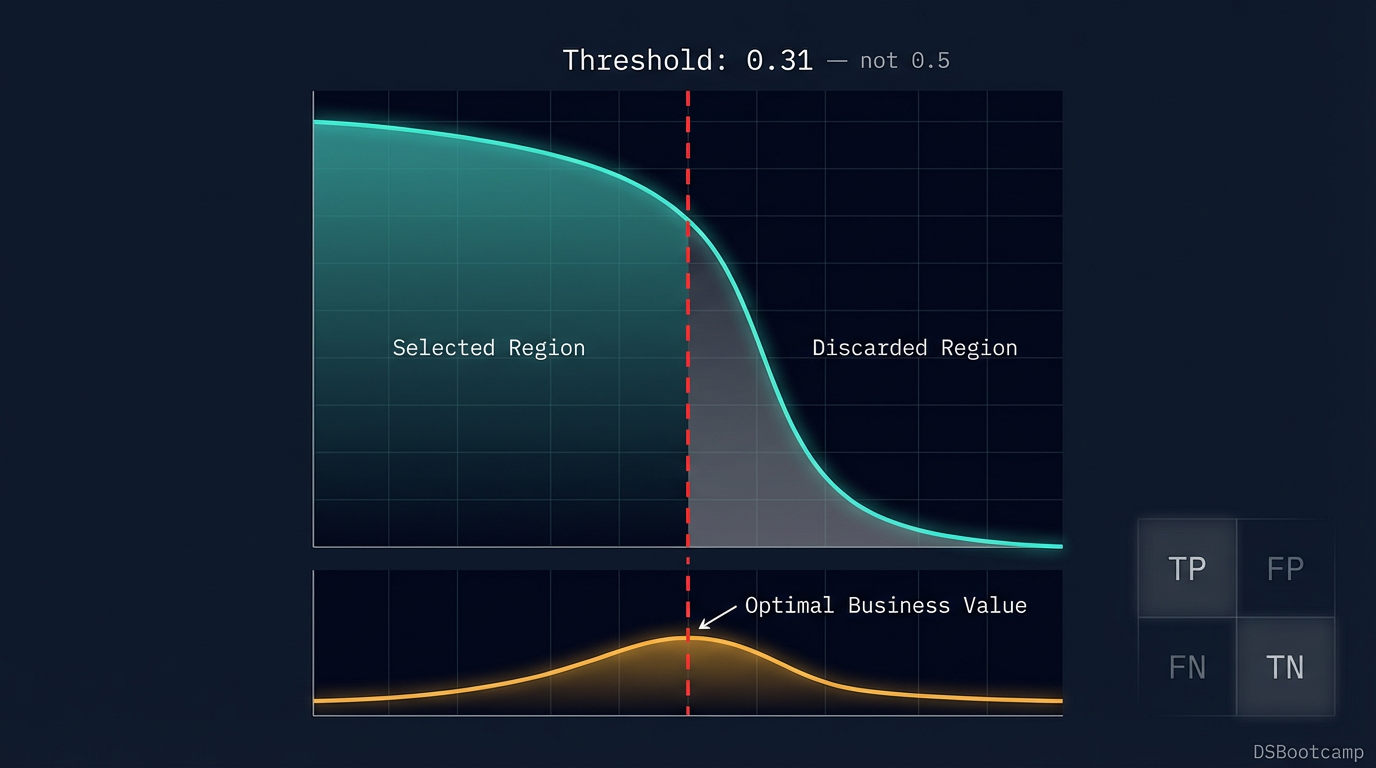
print(f"Recall : {optimal_row['recall']:.3f}")This chart is the artifact that makes the threshold decision a business conversation rather than a technical one. When a stakeholder can see that a threshold of 0.31 generates $147,000 in expected monthly value versus $89,000 at the 0.5 default, the conversation shifts from "why did you change the threshold?" to "why did we ever use 0.5?"
Operational Constraints: The Check That Follows Optimization
The mathematically optimal threshold is your starting point, not your ending point. Production systems have operational constraints that may require adjusting it.
Intervention capacity. If your churn model flags 8,000 customers per week and your retention team can handle 1,500 contacts, the threshold must be set high enough to reduce the flagged population to a manageable volume — even if the cost-optimal threshold would flag 8,000. The constraint isn't mathematical; it's operational. The right framing is: "given that we can contact 1,500 customers per week, what threshold maximizes value on those 1,500?"
# Find threshold that flags at most N customers per week
weekly_volume_cap = 1500
total_customers = len(y_scores)

for _, row in results_df.sort_values('threshold', ascending=False).iterrows():
    flagged = row['TP'] + row['FP']
    if flagged <= weekly_volume_cap:
        print(f"Volume-constrained threshold: {row['threshold']:.2f}")
        print(f"Flagged customers: {flagged}")
        print(f"Expected value: ${row['total_value']:,.0f}")
        break
Regulatory floors. In credit and healthcare, regulators may specify minimum recall thresholds for protected classes or high-risk conditions. A model that is cost-optimal at 82% recall on a medical screening population may be regulatory non-compliant if the floor is 90%. The threshold adjusts upward until the constraint is met, and the business cost of that adjustment is quantified and documented.
Score distribution drift. A threshold set on a validation dataset becomes less reliable as the real-world score distribution shifts over time. Monitor the distribution of model scores monthly and flag when the percentage of scores near the threshold changes significantly — this indicates that a threshold recalibration is warranted, not just periodic model retraining.
Sometimes you need a single metric that encodes the precision-recall tradeoff without requiring a full cost matrix — for instance, when you're comparing multiple candidate models and need a quick scalar evaluation.
The F-beta score gives you this. Beta controls the relative weight given to recall versus precision:
F_β = (1 + β²) × (Precision × Recall) / (β² × Precision + Recall)
When β = 1, you get the standard F1 score — equal weight to precision and recall. When β = 2, recall is weighted twice as heavily as precision. When β = 0.5, precision is weighted more heavily. For fraud detection or medical screening where missing a positive is far more costly, β = 2 is a reasonable default. For spam filtering where false positives (legitimate email flagged as spam) are more damaging than false negatives, β = 0.5 makes more sense.
The F-beta score is a useful shortcut. The cost matrix approach is the right answer. Know which one the situation calls for.
The Step-by-Step Process
Step 1: Build the cost matrix with business stakeholders → Quantify C_TP, C_FP, C_FN before touching any model output
Step 2: Generate probability scores on a held-out validation set → Never set thresholds on training data
Step 3: Plot the precision-recall curve → Evaluate AP score and identify where model confidence lives
Step 4: Compute expected business value across all thresholds → Find the cost-optimal threshold
Step 5: Check operational constraints → Adjust for volume caps, regulatory floors, or SLA requirements
Step 6: Document and present the threshold decision → Show the value curve, the default comparison, and the constraint logic
Step 7: Monitor score distribution in production → Flag when drift warrants threshold recalibration
Seven steps. The default threshold approach skips steps one, three, four, five, and six entirely — which is why it produces suboptimal business outcomes while generating acceptable-looking model metrics.
This post is part of DSBootcamp's Fundamentals series, where we cover the techniques every data scientist needs to know — with the business context, code, and decision frameworks that production work actually demands.