
Part 2 of 3 — Four methods for when you have no clean control group, want to run a real experiment, or need to understand who responds to treatment — not just whether treatment works on average.
Part 1 covered the classical quasi-experimental toolkit: DiD, RDD, IV, and PSM. These methods are powerful when the data structure supports their identifying assumptions. But business problems frequently fall outside those structures — too few treated units for DiD to have adequate power, no threshold to exploit for RDD, no credible instrument, and confounding too severe for PSM to handle.
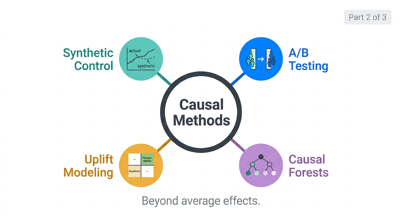
Part 2 covers four methods that extend the toolkit in different directions. Synthetic Control handles the case where you have very few treated units and need to construct a better counterfactual than a simple comparison group provides. A/B Testing is the gold standard when you can actually run the experiment. Uplift Modeling asks a finer question than average treatment effects — who specifically benefits from treatment? And Causal Forests bring the power of machine learning to heterogeneous treatment effect estimation at scale.
Together, these four methods address scenarios that are increasingly common in applied data science but are rarely covered in the same curriculum as their econometric counterparts. They belong in the same toolkit.
Method 5: Synthetic Control
The problem it solves: DiD requires a control group that was trending similarly to the treated group before the intervention. But sometimes you have only one treated unit — one state that adopted a policy, one country that changed a regulation, one major market that got a product launch — and no single comparison unit that matches it well on pre-treatment trends.
The core idea: Instead of choosing a single control unit, construct a weighted combination of control units whose weighted average outcome closely tracks the treated unit's pre-treatment trajectory. This synthetic control becomes the counterfactual for the post-treatment period.
What the weights mean: The synthetic control algorithm finds the combination of untreated units (the "donor pool") that most closely replicates the treated unit's pre-treatment outcome trajectory and, optionally, pre-treatment predictor values. The post-treatment gap between the actual treated unit and the synthetic counterfactual is the causal effect estimate.
The key assumption: The pre-treatment fit quality is the assumption's proxy. If the synthetic control cannot closely match the treated unit's pre-treatment trajectory, the method is not credible for that application. A poor pre-treatment fit is not a sign to proceed with caution — it's a sign the method is inapplicable to this particular problem with the available donor pool.
Best business applications: Market-level interventions where only a small number of markets were treated. Product launch in one city before national rollout. Policy change in one region. Advertising flight in a single DMA. Any setting where N_treated = 1 or very small and rich time-series data exists across many untreated units.
Validation through placebo tests: Run the same synthetic control procedure on each untreated unit in the donor pool, pretending each was treated at the same time. If the actual treated unit shows a post-treatment gap that is substantially larger than the gaps produced by these placebo runs, the finding is not due to chance — a genuine effect is present. This permutation-based inference is the standard validity check for synthetic control.
Method 6: A/B Testing (Randomized Controlled Experiments)
The problem it solves: All quasi-experimental methods rely on assumptions that cannot be verified. The randomized experiment eliminates the need for those assumptions by design — random assignment ensures that treated and control groups are equivalent in expectation on all observed and unobserved characteristics.
A/B testing is not simply "running an experiment." It is a discipline with specific design requirements that are routinely violated in practice, producing misleading results with the same structural confidence as a well-designed test. The failures are almost always in the design phase, not the analysis.
The four most common A/B test failures in production:
Peeking and early stopping — checking results before the pre-specified sample size is reached and stopping when p < 0.05. This inflates the false positive rate from 5% to as high as 30% depending on how many times you peek. Use sequential testing methods if early stopping is operationally required.
Novelty effects — a new feature produces a short-term engagement spike from users who are simply curious. The measured effect during the experiment period overstates the long-term steady-state effect. For features where novelty is plausible, run holdout experiments that measure long-term retention of the treatment effect.
Network effects and SUTVA violations — the Stable Unit Treatment Value Assumption requires that one unit's outcome is unaffected by other units' treatment assignments. In social networks, marketplaces, and any context with user-to-user interaction, this assumption fails. A user whose friends were assigned to the treatment group is contaminated. Use cluster randomization or switchback experiments in these settings.
Metric selection after seeing results — choosing which metric to report based on which one showed significance. Pre-register your primary metric before the experiment launches. Secondary metrics are exploratory.
Best business applications: Product feature releases, UI/UX changes, pricing experiments (where operational constraints allow), onboarding flow optimization, email and notification content tests — any intervention where randomization at the user or session level is feasible.

Method 7: Uplift Modeling
The problem it solves: A/B testing tells you the average treatment effect — whether the intervention works on average across all treated units. But average effects can be deeply misleading for targeting decisions. A retention campaign with a positive average effect might be driven entirely by customers who were going to retain anyway and who just claimed the incentive. The customers who actually changed behavior due to the treatment — the "persuadables" — may be a small fraction of the total.
Uplift modeling directly targets the heterogeneity in treatment effects. Rather than predicting whether a customer will churn, it predicts whether the intervention will change whether the customer churns. This is a fundamentally different model.
The four customer segments that uplift models identify:
- Persuadables: The ones you want to target — they respond positively to treatment
- Sure things: They convert regardless — wasting resources on them adds cost but not value
- Lost causes: They don't respond regardless — targeting adds no value
- Sleeping dogs: Targeting them makes things worse — they would have converted but treatment alienates them.
Validation with the uplift curve and AUUC: Standard classification metrics (AUC, accuracy) are meaningless for evaluating uplift models because you never observe the counterfactual for any individual. Validation uses the uplift curve — plotting cumulative incremental lift as you target progressively larger percentages of the population, ranked by predicted uplift. The Area Under the Uplift Curve (AUUC) summarizes this performance. A random targeting model produces a diagonal; a perfect uplift model curves sharply upward before flattening.
Best business applications: Retention campaigns where some customers would churn regardless and others would retain regardless. Promotional targeting where blanket discounting destroys margin on sure-thing purchasers. Any intervention where the cost of treatment is non-trivial and heterogeneous response is expected.
Method 8: Causal Forests
The problem it solves: Uplift models estimate heterogeneous treatment effects but treat the problem as a standard supervised learning task with ad hoc meta-learning approaches. Causal Forests provide a principled, statistically grounded framework for estimating Conditional Average Treatment Effects (CATE) — the average treatment effect conditional on a specific set of covariate values — with valid confidence intervals.
The core idea: Causal Forests, developed by Wager and Athey (2018), adapt the random forest algorithm to optimize for treatment effect heterogeneity rather than prediction accuracy. Each tree in the forest is built to find splits that maximize the variance of treatment effect estimates across leaves, rather than the variance of the outcome. The honest estimation property — using separate subsamples for tree building and leaf estimation — ensures that confidence intervals are valid.
Why confidence intervals matter for uplift: Without valid uncertainty estimates, you cannot distinguish customers with a genuinely positive treatment effect from customers whose positive uplift score reflects model noise. Causal Forests' confidence intervals let you identify the customers for whom the evidence of a positive effect is statistically credible — a major advance over standard uplift models that produce point estimates with no uncertainty quantification.
Feature importance in causal forests: Unlike standard feature importance, which measures how much a variable improves prediction accuracy, causal forest importance measures how much a variable explains variation in treatment effects across units. This is the correct interpretation for heterogeneous effect analysis — it identifies the subgroup-defining characteristics, not the outcome predictors.
Best business applications: Personalized pricing where individual price sensitivity matters. Targeted interventions where the persuadable population needs to be identified with statistical rigor. Any context where both the direction and magnitude of individual treatment effects are business-critical, and where uncertainty in those estimates should influence targeting decisions.
The Relationship Between These Four Methods
These four methods form a natural progression in terms of the questions they answer and the assumptions they require.
Synthetic Control asks: what would have happened to this treated unit if it hadn't been treated? It requires no randomization but demands rich pre-treatment time-series data and a credible donor pool.
A/B Testing asks: does this treatment work on average, under controlled conditions? It requires the ability to randomize and sufficient traffic/units, but demands fewer assumptions than any observational method.
Uplift Modeling asks: for whom does this treatment work? It requires A/B test data for training and careful validation methodology, but it produces actionable individual-level treatment propensities.
Causal Forests asks: what is the treatment effect for each specific combination of characteristics, and how uncertain are we? It requires A/B test data or strong unconfoundedness assumptions, but it delivers statistically principled heterogeneous effect estimates with valid inference.
A mature business experimentation capability uses all four — Synthetic Control for market-level evaluation, A/B Testing as the baseline experimental discipline, Uplift Modeling for targeting optimization, and Causal Forests when the statistical properties of the effect estimates matter for downstream decisions.
This post is part of DSBootcamp's Econometrics series, where we cover the causal inference methods and statistical frameworks that separate credible business analysis from expensive guesswork.