
The intuition, the parallel trends assumption, and three real business applications where DiD gives you causal estimates without a randomized experiment.
Most business decisions can't be evaluated with a clean randomized experiment. You can't randomly assign half your stores to a new pricing strategy while the other half holds steady for six months — operations won't allow it. You can't randomly assign geographic markets to a new advertising campaign — media buying doesn't work that way. You can't rewind time and ask what revenue would have looked like if you hadn't launched the new loyalty program.
And yet the question you need to answer is always causal: did this intervention actually cause the outcome we observed, or would it have happened anyway?
Difference-in-Differences answers that question from observational data. It's the method that economists use to evaluate minimum wage laws, that policy researchers use to study healthcare reforms, and that increasingly, the best applied data science teams use to evaluate product launches, pricing changes, market expansions, and operational interventions — without a randomized experiment. It is the most practically deployable causal method in the business analytics toolkit, and it is dramatically underused.
The Core Intuition in Two Sentences
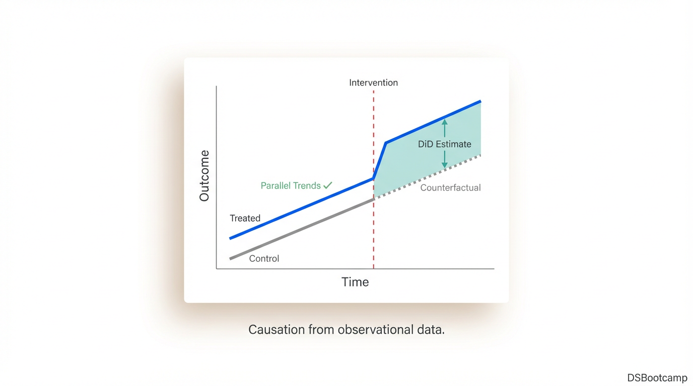
DiD compares the change in outcomes in a treated group before and after an intervention to the change in outcomes in a control group over the same period. The control group's trend provides the counterfactual — what would have happened to the treated group if the intervention had never occurred.
The algebra makes the logic concrete:
DiD Estimate = (Treated_Post − Treated_Pre) − (Control_Post − Control_Pre)
This subtraction does something that a simple before-after comparison on the treated group cannot: it removes the effect of everything that was happening in the world during the same period — macroeconomic trends, seasonality, category-wide shifts, general consumer sentiment — that would have affected both groups equally. What remains is the effect attributable specifically to the intervention.
A Worked Example Before Any Assumptions
Suppose you roll out a new in-store layout to 40 stores in one region while 60 stores in another region continue with the standard layout. Over the same 8-week period:
- Treated stores go from an average of $82,000 weekly revenue to $91,000 — a $9,000 increase
- Control stores go from $79,000 to $84,000 — a $5,000 increase
A naive analyst looks at the treated stores and reports a $9,000 lift from the new layout. But $5,000 of that increase was happening in control stores too — driven by factors completely unrelated to the layout (a seasonal uptick, a successful national promotion, improving consumer confidence). The DiD estimate strips that out:
DiD = ($91,000 − $82,000) − ($84,000 − $79,000) = $9,000 − $5,000 = $4,000
The true causal effect of the new layout is $4,000 per week per store — not $9,000. The naive estimate overstated the impact by 125%. That difference matters enormously when you're deciding whether to invest in rolling out the layout to 300 additional stores.
The Parallel Trends Assumption — The One Thing That Can Break DiD
DiD has one critical identifying assumption: in the absence of the treatment, the treated and control groups would have followed parallel trends. Not identical levels — parallel trajectories. The treated stores don't need to have the same revenue as the control stores. They need to have been changing at the same rate before the intervention.
This assumption cannot be proven for the post-treatment period, because you never observe the counterfactual. But it can be made credible — or shown to be implausible — by examining pre-treatment trends.
import pandas as pd
import matplotlib.pyplot as plt
import statsmodels.formula.api as smf

# Visualize pre-treatment trends for both groups
pre_period = df[df['week'] < intervention_week]

fig, ax = plt.subplots(figsize=(9, 5))
for group, data in pre_period.groupby('treated'):
    label = 'Treated' if group == 1 else 'Control'
    color = 'steelblue' if group == 1 else 'grey'
    weekly_avg = data.groupby('week')['revenue'].mean()
    ax.plot(weekly_avg.index, weekly_avg.values,
            label=label, color=color, lw=2, marker='o')

ax.axvline(intervention_week, color='red', linestyle='--', label='Intervention')
ax.set_title('Pre-Treatment Trends: Parallel Trends Check')
ax.set_xlabel('Week')
ax.set_ylabel('Average Weekly Revenue ($)')
ax.legend()
plt.tight_layout()
plt.show()
If pre-treatment trends are visibly diverging — if the treated group was already pulling away from controls before the intervention — the parallel trends assumption fails, and your DiD estimate is biased. The intervention may have been assigned to already-improving stores, or some other factor was already differentially affecting the two groups.
When pre-trends look parallel, you have a credible design. Plot this before running the regression. Show it in your presentation. It is the single most important diagnostic in any DiD analysis.
Running the DiD Regression
The formal DiD estimate comes from an OLS regression with an interaction term:
Y = β₀ + β₁·Treated + β₂·Post + β₃·(Treated × Post) + ε
Where β₃ is the DiD estimate — the causal effect of the treatment. β₁ captures baseline differences between groups. β₂ captures the time trend common to both groups. The interaction absorbs what's left: the differential change in the treated group attributable to the intervention.
# Create DiD interaction term
df['post'] = (df['week'] >= intervention_week).astype(int)
df['did'] = df['treated'] * df['post']

# Run DiD regression
model = smf.ols('revenue ~ treated + post + did', data=df).fit()
print(model.summary())

# Extract the DiD estimate
did_estimate = model.params['did']
ci_low, ci_high = model.conf_int().loc['did']
print(f"\nDiD Estimate: ${did_estimate:,.0f}")
print(f"95% CI: (${ci_low:,.0f}, ${ci_high:,.0f})")
The regression form is powerful because it extends naturally to include additional controls — store-level fixed effects, week fixed effects, or any covariate that might be driving differential trends. Adding store fixed effects (one binary variable per store) absorbs all time-invariant differences between stores, strengthening the estimate. Adding week fixed effects absorbs all period-specific shocks common across stores. The two-way fixed effects specification — store and week fixed effects together — is the gold standard for panel DiD:
# Two-way fixed effects DiD
model_fe = smf.ols(
'revenue ~ did + C(store_id) + C(week)',
data=df
).fit(cov_type='cluster', cov_kwds={'groups': df['store_id']})

print(f"DiD Estimate (TWFE): ${model_fe.params['did']:,.0f}")
Clustering standard errors by store (the unit of treatment assignment) is non-negotiable. Unclustered standard errors in panel DiD are systematically too small — they understate uncertainty by treating each week-store observation as independent when observations from the same store are correlated over time.
Three Real Business Applications
Application 1: Evaluating a New Store Format Rollout
A retailer pilots a remodeled store format in 25 locations. The remaining 200 stores are unchanged. You have 52 weeks of weekly revenue data per store before the remodel and 26 weeks after. DiD with store and week fixed effects gives you the causal revenue impact of the remodel, controlling for store-level differences and chain-wide trends. This directly informs the business case for investing in the remaining 175 stores.
The parallel trends check here means verifying that the 25 pilot stores weren't already on a stronger revenue trajectory before selection. If pilots were chosen from top-performing stores — a common bias — the treated group may have been already outperforming controls, and the parallel trends assumption fails. Document this selection process and adjust the control group accordingly.
Application 2: Measuring the Impact of a Regional Price Change
Pricing changes are almost never randomized — they're implemented by region or market based on competitive considerations. When a competitor exits a market and you raise prices in that market while holding prices flat elsewhere, DiD lets you estimate the revenue impact of the price change. Treated units are stores in the affected market. Control units are comparable stores in unaffected markets.
The key control group selection decision: "comparable" means stores that were tracking similarly on the relevant metric before the price change, in markets with similar competitive structures. Using all other stores as controls dilutes the estimate if national trends are masking regional variation. Restricting controls to the most similar markets tightens the identifying assumption.
Application 3: Assessing a Policy or Operational Change
An operations team changes dispatch routing logic in a subset of distribution centers as part of a pilot. On-time delivery rate and fulfilment cost are the outcomes. Other DCs operate under the old logic. Weekly operational data for both groups before and after the change gives you a DiD estimate of the policy's causal effect on both metrics simultaneously — running two separate regressions with the same treatment indicator and different outcome variables.
This application is underused in operations analytics specifically because teams tend to evaluate operational changes with simple before-after comparisons at the treated units, ignoring what was happening to the same metrics everywhere else during the same period. Adding the control group comparison is the minimum methodological step that converts an operational report into a defensible causal finding.
The Framing That Makes DiD Credible in Stakeholder Presentations
DiD results land differently depending on how you present them. The frame that works:
"We can't run a randomized experiment on this. But we can ask: what happened to the stores that got the new format relative to what was happening in comparable stores that didn't? If both groups were moving similarly before the change, then the difference in their post-change trajectories is our best estimate of what the format actually caused."
That framing is honest about the method's assumption, clear about what it's doing, and specific about what it's controlling for. It invites productive scrutiny rather than defensive justification. Stakeholders who understand why the control group is there — not as a comparison, but as the counterfactual you otherwise cannot observe — engage with the result at the right level.
DiD doesn't give you the certainty of a randomized experiment. It gives you the best available evidence from the data you actually have. In most business settings, that's exactly what the decision requires.
This post is part of DSBootcamp's Statistics series, where we cover the causal inference methods and statistical frameworks that separate credible business analysis from expensive guesswork.